aCompCor for line-scanning
This notebook illustrates how to anatomical component correction (aCompCor) on line-scanning data. Though this may seem trivial on regular whole-brain fMRI data, the effect of aCompCor on line-scanning data is quite pronounced and therefore worthy of its own example notebook. We’ll then also perform a quick analysis, and you can compare the results with the nideconv example.
[14]:
%matplotlib inline
[4]:
# imports
from linescanning import (
    dataset,
    plotting,
    utils,
    fitting
    )
import warnings
import os
import matplotlib.pyplot as plt
from scipy.io import loadmat
from sklearn.metrics import r2_score
import seaborn as sns
opj = os.path.join

warnings.simplefilter('ignore')
project_dir = os.environ.get("DIR_PROJECTS")
base_dir = opj(project_dir, 'hemifield')
deriv_dir = opj(base_dir, 'derivatives')

plot_vox = 359
plot_xkcd = False
For aCompCor, we need some preparation steps before we can load everything in. We need the following:
A registration matrix mapping ``ses-1`` to the line-scanning session (e.g., ``ses-3``); this one is generally obtained during the planning of the line with
spinoza_lineplanning, but can be tailored to be closer to the first anatomical slice. For instance, we often acquiremulti-sliceimages inbetween runs. Given that these images are often closer the line-scanning run, you can usecall_ses1_to_motion1to create a matrix mappingses-1to the first anatomical slice.Transformations mapping run-to-run; the matrix above deals with session-to-session registration, but not motion inbetween runs. We can not see every bit of motion due to the 2D-nature of the data, but we can do our best. To get these registration matrices I use
ITK-Snap. We’ll definerun-1as moving run, and the subsequent runs as reference runs. This means we need to open the reference images asmainimage in ITK-Snap, and the run-1 slice (moving) as overlay. PressTools>Registration>Manualand align the slices to the best of your abilities. Then save the matrix by pressing thesaveicon on the bottom left as:from-run1_to-run<run_ID>.txtin theanat-folder of your line-scanning session
Now we have the ingredients to do aCompCor. For each run, the segmentations of ses-1 will be transformed to the particular run using the 2 matrices provided (providing only 1 will lead to inaccurate alignment). We then perform PCA on the WM/CSF voxel timecourses. To eliminate the possibility of filtering out task-related frequencies, we high-pass the resulting components, before regressing them out. This is all done for you within the linescanning.Dataset-class.
[5]:
# Load data
sub         = '003'
ses         = 3
task        = "task-SR"
runs        = [3,4,6]
func_dir    = opj(base_dir, f"sub-{sub}", f"ses-{ses}", "func")
anat_dir    = opj(os.path.dirname(func_dir), 'anat')
ribbon      = (356,363)

run_files   = utils.get_file_from_substring([f"sub-{sub}", f"ses-{ses}", f"{task}"], func_dir)
func_file   = utils.get_file_from_substring("bold.mat", run_files)
exp_file    = utils.get_file_from_substring("events.tsv", run_files)
anat_slices = utils.get_file_from_substring([f"sub-{sub}", f"ses-{ses}", "acq-1slice", ".nii.gz"], anat_dir)
ref_slices  = utils.match_lists_on(func_file, anat_slices, matcher='run')
ref_slices
[5]:
['/data1/projects/MicroFunc/Jurjen/projects/hemifield/sub-003/ses-3/anat/sub-003_ses-3_acq-1slice_run-3_T1w.nii.gz',
 '/data1/projects/MicroFunc/Jurjen/projects/hemifield/sub-003/ses-3/anat/sub-003_ses-3_acq-1slice_run-4_T1w.nii.gz',
 '/data1/projects/MicroFunc/Jurjen/projects/hemifield/sub-003/ses-3/anat/sub-003_ses-3_acq-1slice_run-6_T1w.nii.gz']
Now we insert everything again in dataset as before, but now you’ll see it outputs plots regarding the effect of aCompCor on the data
[7]:
# mind you, the segmentations live in ses-1 space, NOT FREESURFER!
ses_to_motion = utils.get_file_from_substring(f"ses{ses}_rec-motion1", opj(deriv_dir, 'pycortex', f"sub-{sub}", 'transforms'))
run2run = utils.get_file_from_substring(['.txt'], anat_dir)

# initiate object
data_obj = dataset.Dataset(
    func_file,
    tsv_file=exp_file,
    deleted_first_timepoints=50,
    deleted_last_timepoints=50,
    use_bids=True,
    verbose=True,
    acompcor=True,
    ref_slice=ref_slices,
    ses1_2_ls=ses_to_motion,
    run_2_run=run2run,
    n_pca=5,
    report=False)

df_func     = data_obj.fetch_fmri()
df_onsets   = data_obj.fetch_onsets()
df_onsets
DATASET

FUNCTIONAL
Preprocessing /data1/projects/MicroFunc/Jurjen/projects/hemifield/sub-003/ses-3/func/sub-003_ses-3_task-SR_run-3_bold.mat
 Filtering strategy: 'hp'
 Standardization strategy: 'psc'
 Baseline is 20 seconds, or 190 TRs
 Cutting 50 volumes from beginning (also cut from baseline (was 190, now 140 TRs)
 DCT-high pass filter [removes low frequencies <0.01 Hz] to correct low-frequency drifts.
 Reading /data1/projects/MicroFunc/Jurjen/projects/VE-pRF/derivatives/nighres/sub-003/ses-3/sub-003_ses-3_run-3_desc-segmentations.pkl
 Found 25 voxel for nuisance regression; (indices<300 are ignored due to distance from coil)
 We're good to go!
 Using 5 components for aCompCor (WM/CSF separately)
 Found 1 component(s) in 'csf'-voxels with total explained variance of 0.6%
 Found 1 component(s) in 'wm'-voxels with total explained variance of 0.45%
 DCT high-pass filter on components [removes low frequencies <0.2 Hz]
 tSNR [before 'acompcor']: 18.57        | variance: 0.76
 tSNR [after 'acompcor']:  22.05        | variance: 0.4
Preprocessing /data1/projects/MicroFunc/Jurjen/projects/hemifield/sub-003/ses-3/func/sub-003_ses-3_task-SR_run-4_bold.mat
 Filtering strategy: 'hp'
 Standardization strategy: 'psc'
 Baseline is 20 seconds, or 190 TRs
 Cutting 50 volumes from beginning (also cut from baseline (was 190, now 140 TRs)
 DCT-high pass filter [removes low frequencies <0.01 Hz] to correct low-frequency drifts.
 Reading /data1/projects/MicroFunc/Jurjen/projects/VE-pRF/derivatives/nighres/sub-003/ses-3/sub-003_ses-3_run-4_desc-segmentations.pkl
 Found 28 voxel for nuisance regression; (indices<300 are ignored due to distance from coil)
 We're good to go!
 Using 5 components for aCompCor (WM/CSF separately)
 Found 1 component(s) in 'csf'-voxels with total explained variance of 0.51%
 Found 1 component(s) in 'wm'-voxels with total explained variance of 0.46%
 DCT high-pass filter on components [removes low frequencies <0.2 Hz]
 tSNR [before 'acompcor']: 19.9 | variance: 0.7
 tSNR [after 'acompcor']:  23.67        | variance: 0.38
Preprocessing /data1/projects/MicroFunc/Jurjen/projects/hemifield/sub-003/ses-3/func/sub-003_ses-3_task-SR_run-6_bold.mat
 Filtering strategy: 'hp'
 Standardization strategy: 'psc'
 Baseline is 20 seconds, or 190 TRs
 Cutting 50 volumes from beginning (also cut from baseline (was 190, now 140 TRs)
 DCT-high pass filter [removes low frequencies <0.01 Hz] to correct low-frequency drifts.
 Reading /data1/projects/MicroFunc/Jurjen/projects/VE-pRF/derivatives/nighres/sub-003/ses-3/sub-003_ses-3_run-6_desc-segmentations.pkl
 Found 21 voxel for nuisance regression; (indices<300 are ignored due to distance from coil)
 We're good to go!
 Using 5 components for aCompCor (WM/CSF separately)
 Found 1 component(s) in 'csf'-voxels with total explained variance of 0.56%
 Found 1 component(s) in 'wm'-voxels with total explained variance of 0.46%
 DCT high-pass filter on components [removes low frequencies <0.2 Hz]
 tSNR [before 'acompcor']: 22.81        | variance: 0.51
 tSNR [after 'acompcor']:  27.01        | variance: 0.36

EXPTOOLS
Preprocessing /data1/projects/MicroFunc/Jurjen/projects/hemifield/sub-003/ses-3/func/sub-003_ses-3_task-SR_run-3_events.tsv
 1st 't' @153.63s
 Cutting 158.88s from onsets
Preprocessing /data1/projects/MicroFunc/Jurjen/projects/hemifield/sub-003/ses-3/func/sub-003_ses-3_task-SR_run-4_events.tsv
 1st 't' @109.93s
 Cutting 115.18s from onsets
Preprocessing /data1/projects/MicroFunc/Jurjen/projects/hemifield/sub-003/ses-3/func/sub-003_ses-3_task-SR_run-6_events.tsv
 1st 't' @117.54s
 Cutting 122.79s from onsets

DATASET: created
Fetching dataframe from attribute 'df_func_acomp'
[7]:
| onset | |||
|---|---|---|---|
| subject | run | event_type | |
| 003 | 3 | 2.014613132977678 | 24.363776 |
| 3.5652478065289 | 35.213706 | ||
| 2.13914868391734 | 39.913720 | ||
| 3.5652478065289 | 47.413652 | ||
| 2.014613132977678 | 53.213640 | ||
| ... | ... | ... | |
| 6 | 1.140879298089248 | 373.028252 | |
| 1.853928859395028 | 378.111696 | ||
| 1.140879298089248 | 382.953138 | ||
| 2.13914868391734 | 387.653167 | ||
| 2.014613132977678 | 394.244731 |
150 rows × 1 columns
For each run, the following is plotted:
The WM (red) and CSF (blue) voxels used for PCA
The scree plot of WM/CSF
The power spectra of the selected components
The power spectra of a real voxel timecourse before (green) and after (orange) aCompCor
You should be able to see that breathing-related frequencies (~0.25-0.3Hz) and cardiac frequencies (~1Hz) are largely removed. Now we’re back with a dataframe that we can use with NideconvFitter as before
We can save the object as an h5-file
[6]:
data_obj.to_hdf()
---------------------------------------------------------------------------
ValueError                                Traceback (most recent call last)
/tmp/ipykernel_692/1612606920.py in <module>
----> 1 data_obj.to_hdf()

/mnt/d/FSL/shared/spinoza/programs/packages/linescanning/linescanning/dataset.py in to_hdf(self, output_file, overwrite)
   2295                 self.h5_file = opj(self.lsprep_full, "dataset.h5")
   2296             else:
-> 2297                 raise ValueError("No output file specified")
   2298         else:
   2299             self.h5_file = output_file

ValueError: No output file specified
And read from that file later on
[7]:
data_obj2 = dataset.Dataset(data_obj.h5_file)
df_func2 = data_obj2.fetch_fmri()
df_func2.head()
[7]:
| vox 0 | vox 1 | vox 2 | vox 3 | vox 4 | vox 5 | vox 6 | vox 7 | vox 8 | vox 9 | ... | vox 710 | vox 711 | vox 712 | vox 713 | vox 714 | vox 715 | vox 716 | vox 717 | vox 718 | vox 719 | |||
|---|---|---|---|---|---|---|---|---|---|---|---|---|---|---|---|---|---|---|---|---|---|---|---|
| subject | run | t | |||||||||||||||||||||
| 003 | 3 | 0.000 | -11.268791 | 20.675842 | 3.643059 | 5.464417 | 19.831787 | -1.580231 | -5.665932 | 8.045868 | 1.001884 | 7.231850 | ... | -6.231232 | 1.926201 | -26.192245 | 10.043640 | 19.279381 | 37.216156 | -5.807785 | -36.261780 | -38.368538 | 8.164024 |
| 0.105 | 5.220299 | 3.646629 | 1.561874 | -18.175636 | 11.372185 | 13.392868 | 1.031944 | 4.021049 | -7.899956 | -0.733025 | ... | 37.002457 | -0.116684 | 54.194107 | 65.822792 | 25.281830 | -16.733543 | 43.018570 | 45.518127 | -25.205460 | -20.410423 | ||
| 0.210 | 16.124245 | 4.645760 | -9.609238 | 14.061096 | 3.064301 | 14.061806 | 1.619110 | -9.753319 | 7.980743 | -4.526749 | ... | 17.694405 | -38.169361 | -25.722763 | 21.115028 | 26.644882 | -31.216881 | -13.721283 | -7.407021 | -85.227013 | 17.002090 | ||
| 0.315 | 0.274521 | 2.146027 | 9.739418 | 11.125603 | 2.868805 | 16.629951 | 14.436333 | 3.256439 | -2.695702 | 8.151466 | ... | -20.756516 | 29.955048 | -2.776077 | -12.668266 | 9.367783 | -1.626862 | 29.095657 | 36.880600 | -31.587967 | 8.983261 | ||
| 0.420 | 0.011894 | -12.099632 | -4.228523 | 20.763100 | -2.864799 | 4.398376 | 2.538567 | 1.098625 | 10.500237 | 5.553429 | ... | 14.928970 | 0.116684 | -42.732121 | -1.089157 | 32.637619 | -20.906685 | 12.145576 | -47.056499 | -35.285698 | -22.710487 |
5 rows × 720 columns
And we see it’s the same as the original dataframe
[8]:
df_func.head()
[8]:
| vox 0 | vox 1 | vox 2 | vox 3 | vox 4 | vox 5 | vox 6 | vox 7 | vox 8 | vox 9 | ... | vox 710 | vox 711 | vox 712 | vox 713 | vox 714 | vox 715 | vox 716 | vox 717 | vox 718 | vox 719 | |||
|---|---|---|---|---|---|---|---|---|---|---|---|---|---|---|---|---|---|---|---|---|---|---|---|
| subject | run | t | |||||||||||||||||||||
| 003 | 3 | 0.000 | -11.268791 | 20.675842 | 3.643059 | 5.464417 | 19.831787 | -1.580231 | -5.665932 | 8.045876 | 1.001884 | 7.231842 | ... | -6.231232 | 1.926201 | -26.192245 | 10.043640 | 19.279373 | 37.216156 | -5.807785 | -36.261780 | -38.368546 | 8.164024 |
| 0.105 | 5.220299 | 3.646629 | 1.561874 | -18.175636 | 11.372185 | 13.392868 | 1.031944 | 4.021049 | -7.899956 | -0.733032 | ... | 37.002457 | -0.116684 | 54.194107 | 65.822792 | 25.281830 | -16.733543 | 43.018570 | 45.518127 | -25.205467 | -20.410423 | ||
| 0.210 | 16.124245 | 4.645760 | -9.609238 | 14.061096 | 3.064301 | 14.061806 | 1.619110 | -9.753319 | 7.980743 | -4.526756 | ... | 17.694405 | -38.169361 | -25.722763 | 21.115028 | 26.644882 | -31.216881 | -13.721283 | -7.407021 | -85.227020 | 17.002090 | ||
| 0.315 | 0.274521 | 2.146027 | 9.739418 | 11.125603 | 2.868805 | 16.629951 | 14.436333 | 3.256439 | -2.695702 | 8.151459 | ... | -20.756516 | 29.955048 | -2.776077 | -12.668266 | 9.367783 | -1.626862 | 29.095657 | 36.880585 | -31.587975 | 8.983261 | ||
| 0.420 | 0.011894 | -12.099632 | -4.228523 | 20.763100 | -2.864799 | 4.398376 | 2.538567 | 1.098625 | 10.500237 | 5.553421 | ... | 14.928970 | 0.116684 | -42.732121 | -1.089157 | 32.637619 | -20.906685 | 12.145576 | -47.056499 | -35.285706 | -22.710487 |
5 rows × 720 columns
[8]:
df_ribbon = utils.select_from_df(df_func, expression='ribbon', indices=ribbon)
df_ribbon
[8]:
| vox 356 | vox 357 | vox 358 | vox 359 | vox 360 | vox 361 | vox 362 | |||
|---|---|---|---|---|---|---|---|---|---|
| subject | run | t | |||||||
| 003 | 3 | 0.000 | 1.291512 | 1.673363 | 1.014069 | -2.534813 | -3.339218 | -5.837639 | -4.163383 |
| 0.105 | -0.447891 | -1.858551 | -0.716454 | 0.316788 | 0.699730 | 1.557922 | 2.709099 | ||
| 0.210 | -0.154091 | 1.333786 | 2.301636 | 0.543060 | -2.958778 | -2.669579 | -1.719719 | ||
| 0.315 | 0.172256 | -0.484093 | 1.191910 | -2.388977 | 0.547096 | -2.186348 | 1.335541 | ||
| 0.420 | 2.191238 | 2.933685 | 0.419159 | 2.834633 | -0.912849 | 1.509354 | -1.473938 | ||
| ... | ... | ... | ... | ... | ... | ... | ... | ... | |
| 6 | 450.975 | -0.236420 | 1.703430 | -0.970009 | 0.522400 | -1.332176 | 1.864960 | 0.403328 | |
| 451.080 | 3.710991 | -0.338005 | 2.691170 | 2.280724 | 2.631653 | 0.467560 | -0.265839 | ||
| 451.185 | -1.374130 | 2.831108 | 1.778114 | 0.244553 | 0.808685 | 3.256584 | 0.594902 | ||
| 451.290 | 4.197334 | -0.125290 | 1.121887 | 2.262886 | 2.393730 | -0.269264 | 0.664070 | ||
| 451.395 | -0.605896 | -0.387215 | 0.771248 | 0.216942 | 1.775826 | 1.373344 | 1.178215 |
13300 rows × 7 columns
Right, on to the fitting: we can do the fitting with utils.NideconvFitter, which requires the functional dataframe, onset dataframe, and some settings on the type of fit you’d like to do, number of regressors, confounds, etc.
[9]:
# we can fit with canonical HRFs
interval = [0,20]
nd_gamma = fitting.NideconvFitter(
    df_ribbon,
    df_onsets,
    confounds=None,
    basis_sets='canonical_hrf_with_time_derivative',
    n_regressors=None,
    lump_events=False,
    TR=0.105,
    interval=interval,
    add_intercept=True,
    verbose=True)
Selected 'canonical_hrf_with_time_derivative'-basis sets
Adding event '1.140879298089248' to model
Adding event '1.853928859395028' to model
Adding event '2.014613132977678' to model
Adding event '2.13914868391734' to model
Adding event '3.5652478065289' to model
Fitting with 'ols' minimization
Done
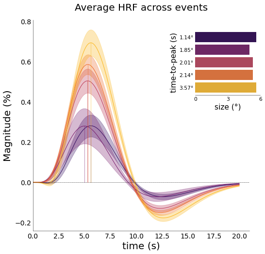
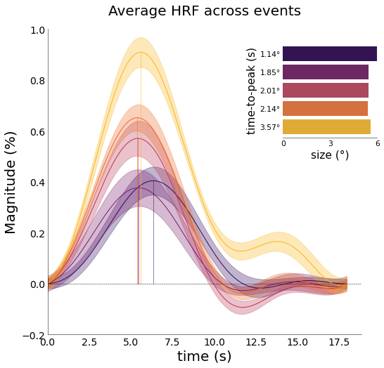
[48]:
# instantiating figure allows insets to be saved too
font_size = 20
fig,axs = plt.subplots(figsize=(8,8))
nd_gamma.plot_average_per_event(
    font_size=font_size,
    axs=axs ,
    x_label="time (s)",
    y_label="Magnitude (%)",
    add_hline='default',
    ttp=True,
    ttp_lines=True,
    add_labels=True,
    y_label2="time-to-peak (s)",
    x_label2="size (°)",
    ttp_labels=[f"{round(float(ii),2)}°" for ii in nd_gamma.cond],
    lim=[0,6],
    ticks=[0,3,6],
    cmap='inferno')
# fig.savefig(opj(func_dir, "hrf_events_ttp.png"), dpi=300, bbox_inches='tight')
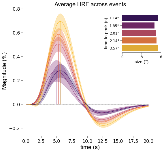
[204]:
# instantiating figure allows insets to be saved too
font_size = 20
fig,axs = plt.subplots(figsize=(8,8))
nd_gamma.plot_average_per_event(
    xkcd=False,
    alpha=0.2,
    font_size=font_size,
    axs=axs ,
    x_label="time (s)",
    y_label="Magnitude (%)",
    add_hline='default',
    ttp=True,
    ttp_lines=True,
    add_labels=True,
    y_label2="time-to-peak (s)",
    x_label2="size (°)",
    ttp_labels=[f"{round(float(ii),2)}°" for ii in nd_gamma.cond],
    lim=[0, 6],
    ticks=[0, 3, 6],
    cmap='inferno')
fig.savefig(opj(func_dir, "hrf_events_ttp.png"), dpi=300, bbox_inches='tight')
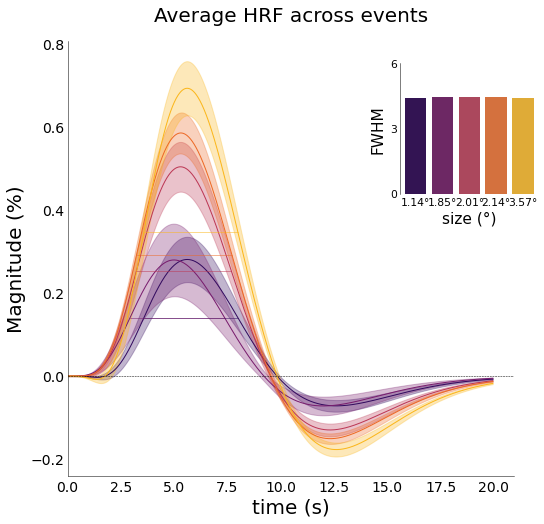
[49]:
# instantiating figure allows insets to be saved too
fig,axs = plt.subplots(figsize=(8,8))
nd_gamma.plot_average_per_event(
    xkcd=False,
    font_size=font_size,
    axs=axs ,
    x_label="time (s)",
    y_label="Magnitude (%)",
    add_hline='default',
    fwhm=True,
    fwhm_lines=True,
    add_labels=True,
    y_label2="FWHM",
    x_label2="size (°)",
    fwhm_labels=[f"{round(float(ii),2)}°" for ii in nd_gamma.cond],
    lim=[0, 6],
    ticks=[0, 3, 6],
    cmap='inferno')
# fig.savefig(opj(func_dir, "hrf_events_fwhm.png"), dpi=300, bbox_inches='tight')
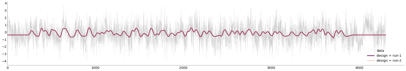
Here we consider the predictions that arise from the deconvolved HRF
[42]:
colors = sns.color_palette('inferno', 2)
cross_pred = nd_gamma.fitters.iloc[0].X.dot(nd_gamma.fitters.iloc[0].betas)

plotting.LazyPlot(
    [utils.select_from_df(df_ribbon, expression="run = 3").iloc[:,0].values,
    utils.select_from_df(nd_gamma.predictions, expression="run = 3").iloc[:,0].values,
    cross_pred.iloc[:,0].values],
    line_width=[0.5,3,1],
    color=["#cccccc"]+colors,
    labels=["data", "design = run-1", "design = run-2"])
0
[42]:
<linescanning.plotting.LazyPlot at 0x7f9be30a18e0>
[43]:
# individual model fits
fit_objs = []
for ii in nd_gamma.cond:

    nd_fit = fitting.NideconvFitter(
        df_ribbon,
        utils.select_from_df(df_onsets, expression=f"event_type = {ii}"),
        confounds=None,
        basis_sets='canonical_hrf_with_time_derivative',
        n_regressors=None,
        lump_events=False,
        TR=0.105,
        interval=[0,18],
        add_intercept=True,
        verbose=True)

    nd_fit.timecourses_condition()
    fit_objs.append(nd_fit)
Selected 'canonical_hrf_with_time_derivative'-basis sets
Adding event '1.140879298089248' to model
Fitting with 'ols' minimization
Done
Selected 'canonical_hrf_with_time_derivative'-basis sets
Adding event '1.853928859395028' to model
Fitting with 'ols' minimization
Done
Selected 'canonical_hrf_with_time_derivative'-basis sets
Adding event '2.014613132977678' to model
Fitting with 'ols' minimization
Done
Selected 'canonical_hrf_with_time_derivative'-basis sets
Adding event '2.13914868391734' to model
Fitting with 'ols' minimization
Done
Selected 'canonical_hrf_with_time_derivative'-basis sets
Adding event '3.5652478065289' to model
Fitting with 'ols' minimization
Done
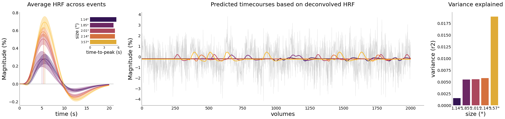
[64]:
fig = plt.figure(figsize=(30,6))
gs = fig.add_gridspec(1,3, width_ratios=[1,3,0.5], wspace=0.2)
font_size = 20

ax1 = fig.add_subplot(gs[0])
nd_gamma.plot_average_per_event(
    axs=ax1,
    x_label="time (s)",
    y_label="Magnitude (%)",
    add_hline='default',
    ttp=True,
    ttp_lines=True,
    add_labels=True,
    y_label2="size (°)",
    x_label2="time-to-peak (s)",
    ttp_labels=[f"{round(float(ii),2)}°" for ii in nd_gamma.cond],
    lim=[0, 6],
    ticks=[0,3,6],
    cmap='inferno',
    font_size=font_size)

ax2 = fig.add_subplot(gs[1])
colors = sns.color_palette('inferno', len(nd_gamma.cond))
preds = [utils.select_from_df(fit_objs[ii].predictions, expression="run = 3").iloc[:,0].values for ii in range(len(fit_objs))]
real = utils.select_from_df(df_ribbon, expression="run = 3").iloc[:, 0].values

plotting.LazyPlot(
    [ii[:2000] for ii in [real]+preds],
    line_width=[0.5]+[2 for ii in range(len(fit_objs))],
    color=["#cccccc"]+colors,
    axs=ax2,
    title="Predicted timecourses based on deconvolved HRF",
    font_size=font_size,
    x_label="volumes",
    y_label="Magnitude (%)")

# calculate r2's
ax3 = fig.add_subplot(gs[2])
r2s = [r2_score(real, preds[ii]) for ii in range(len(fit_objs))]
plotting.LazyBar(
    x=[f"{round(float(ii),2)}°" for ii in nd_gamma.cond],
    y=r2s,
    palette=colors,
    sns_ori="v",
    axs=ax3,
    add_labels=True,
    x_label2="size (°)",
    y_label2="variance (r2)",
    font_size=font_size,
    title2="Variance explained")

# fig.savefig(opj(func_dir, "r2_score.png"))
[64]:
<linescanning.plotting.LazyBar at 0x7f9be33c5310>
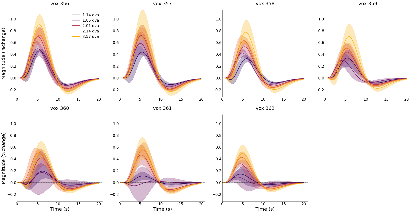
[65]:
nd_gamma.plot_average_per_voxel(
    labels=[f"{round(float(ii),2)} dva" for ii in nd_gamma.cond],
    wspace=0.2,
    cmap="inferno",
    line_width=2,
    font_size=font_size,
    label_size=16,
    sharey=True)
    # save_as=opj(func_dir, "hrf_gamma_voxel.png"))
[66]:
nd_gamma.cond
[66]:
array(['1.140879298089248', '1.853928859395028', '2.014613132977678',
       '2.13914868391734', '3.5652478065289'], dtype='<U17')
[68]:
nd_gamma.arr_voxels_in_event[0,...].shape
[68]:
(5, 3800)
[69]:
cross_pred = nd_gamma.fitters.iloc[0].predict_from_design_matrix(X=nd_gamma.fitters.iloc[1].X)
cross_pred
[69]:
| prediction for vox 356 | prediction for vox 357 | prediction for vox 358 | prediction for vox 359 | prediction for vox 360 | prediction for vox 361 | prediction for vox 362 | |
|---|---|---|---|---|---|---|---|
| time | |||||||
| 0.000 | -0.411264 | -0.409654 | -0.364163 | -0.130388 | -0.224184 | 0.117909 | 0.189639 |
| 0.105 | -0.411264 | -0.409654 | -0.364163 | -0.130388 | -0.224184 | 0.117909 | 0.189639 |
| 0.210 | -0.411264 | -0.409654 | -0.364163 | -0.130388 | -0.224184 | 0.117909 | 0.189639 |
| 0.315 | -0.411264 | -0.409654 | -0.364163 | -0.130388 | -0.224184 | 0.117909 | 0.189639 |
| 0.420 | -0.411264 | -0.409654 | -0.364163 | -0.130388 | -0.224184 | 0.117909 | 0.189639 |
| ... | ... | ... | ... | ... | ... | ... | ... |
| 450.975 | -0.411264 | -0.409654 | -0.364163 | -0.130388 | -0.224184 | 0.117909 | 0.189639 |
| 451.080 | -0.411264 | -0.409654 | -0.364163 | -0.130388 | -0.224184 | 0.117909 | 0.189639 |
| 451.185 | -0.411264 | -0.409654 | -0.364163 | -0.130388 | -0.224184 | 0.117909 | 0.189639 |
| 451.290 | -0.411264 | -0.409654 | -0.364163 | -0.130388 | -0.224184 | 0.117909 | 0.189639 |
| 451.395 | -0.411264 | -0.409654 | -0.364163 | -0.130388 | -0.224184 | 0.117909 | 0.189639 |
4300 rows × 7 columns
[70]:
# we can fit with fourier
nd_fourier = fitting.NideconvFitter(
    df_ribbon,
    df_onsets,
    confounds=None,
    basis_sets='fourier',
    n_regressors=4,
    lump_events=False,
    TR=0.105,
    interval=[0,18],
    add_intercept=True,
    verbose=True)
Selected 'fourier'-basis sets
Adding event '1.140879298089248' to model
Adding event '1.853928859395028' to model
Adding event '2.014613132977678' to model
Adding event '2.13914868391734' to model
Adding event '3.5652478065289' to model
Fitting with 'ols' minimization
Done
[71]:
nd_fourier.plot_average_per_event(
    xkcd=False,
    figsize=(8, 8),
    x_label="time (s)",
    y_label="Magnitude (%)",
    add_hline='default',
    y_lim=[-0.2,1],
    ttp=True,
    ttp_lines=True,
    add_labels=True,
    y_label2="time-to-peak (s)",
    x_label2="size (°)",
    ttp_labels=[f"{round(float(ii),2)}°" for ii in nd_fourier.cond],
    lim=[0, 6],
    ticks=[0, 3, 6],
    cmap='inferno',
    save_as=opj(func_dir, "hrf_fourier.png"),
    font_size=font_size)
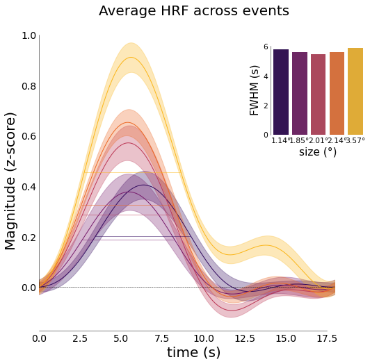
[73]:
nd_fourier.plot_average_per_event(
    xkcd=False,
    x_label="time (s)",
    y_label="Magnitude (z-score)",
    add_hline='default',
    sns_trim=True,
    fwhm=True,
    fwhm_lines=True,
    fwhm_labels=[f"{round(float(ii),2)}°" for ii in nd_fourier.cond],
    add_labels=True,
    x_label2="size (°)",
    y_label2="FWHM (s)",
    cmap='inferno',
    font_size=font_size)
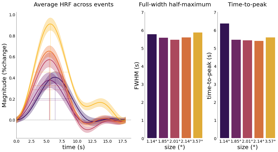
[76]:
fig = plt.figure(figsize=(16,8))
gs = fig.add_gridspec(1,3, width_ratios=[2,1,1])

ax = fig.add_subplot(gs[0])
nd_fourier.plot_average_per_event(
    axs=ax,
    x_label="time (s)",
    y_label="Magnitude (%change)",
    add_hline='default',
    line_width=2,
    font_size=font_size,
    cmap='inferno')

ax2 = fig.add_subplot(gs[1])
nd_fourier.plot_fwhm(
    nd_fourier.event_avg,
    axs=ax2,
    hrf_axs=ax,
    fwhm_labels=[f"{round(float(ii),2)}°" for ii in nd_fourier.cond],
    x_label2="size (°)",
    y_label2="FWHM (s)",
    title2="Full-width half-maximum",
    add_labels=True,
    font_size=font_size,
    lim=[0, 7],
    fwhm_lines=True,
    sns_offset=5)

ax3 = fig.add_subplot(gs[2])
nd_fourier.plot_ttp(
    nd_fourier.event_avg,
    axs=ax3,
    hrf_axs=ax,
    ttp_labels=[f"{round(float(ii),2)}°" for ii in nd_fourier.cond],
    y_label2="time-to-peak (s)",
    x_label2="size (°)",
    title2="Time-to-peak",
    add_labels=True,
    font_size=font_size,
    lim=[0,7],
    ttp_lines=True,
    sns_offset=5,
    ttp_ori='v')
[78]:
nd_fourier.plot_average_per_voxel(
    labels=[f"{round(float(ii),2)} dva" for ii in nd_fourier.cond],
    wspace=0.2,
    cmap="inferno",
    line_width=2,
    sharey=True)
    # save_as=opj(func_dir, "hrf_fourier_voxel.png"))
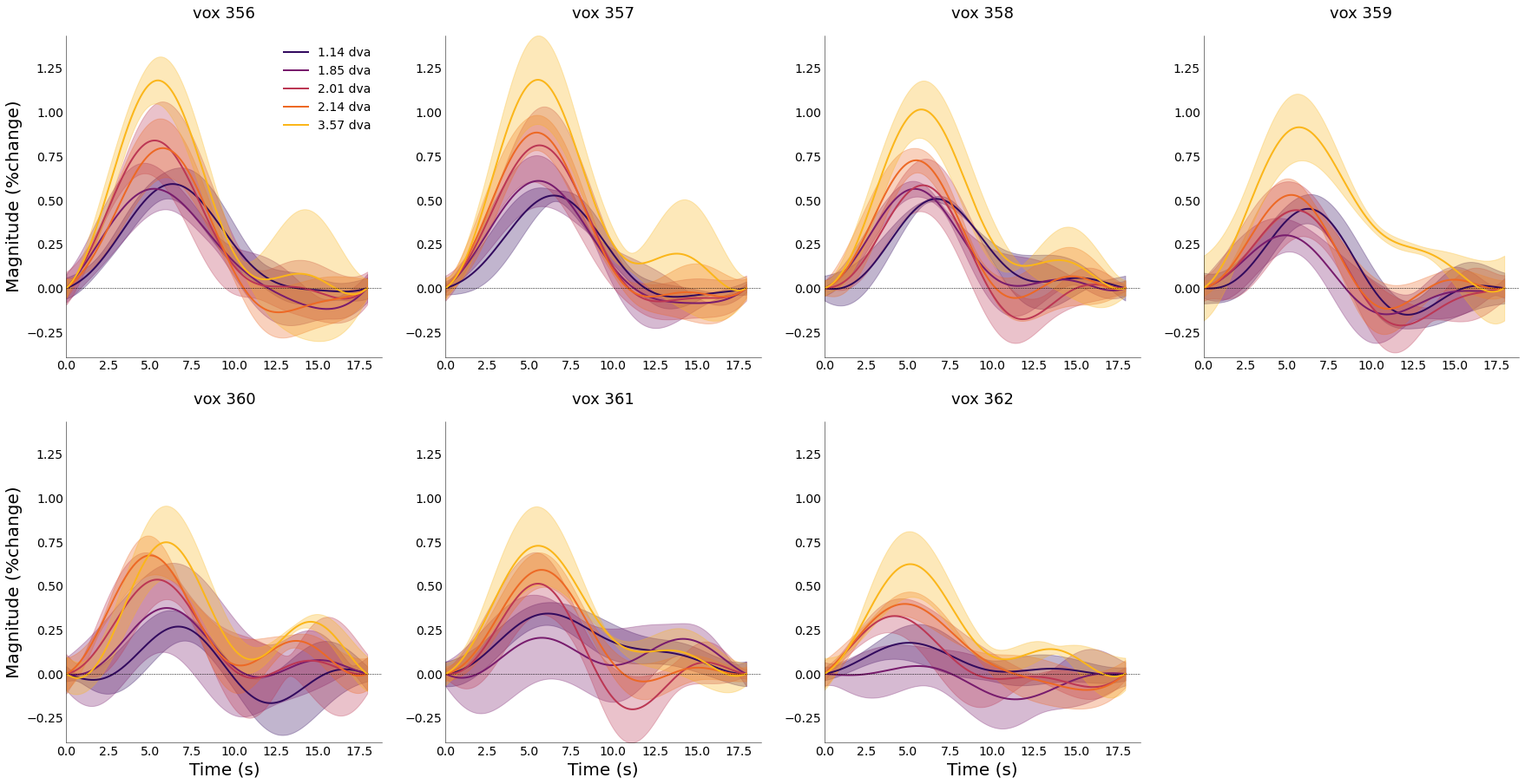
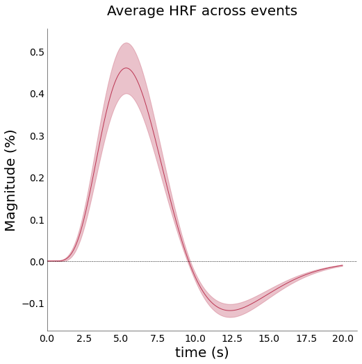
The models above considered each stimulus event (stimulus size) as separate event. Again, we can also lump them together into a single event to get an average HRF
[79]:
lumped = fitting.NideconvFitter(
    df_ribbon,
    df_onsets,
    confounds=None,
    basis_sets='canonical_hrf_with_time_derivative',
    n_regressors=4,
    lump_events=True,
    TR=0.105,
    interval=interval,
    add_intercept=True,
    verbose=True,
    fit_type='ols')

lumped.plot_average_per_event(
    figsize=(8,8),
    x_label="time (s)",
    y_label="Magnitude (%)",
    add_hline='default',
    font_size=font_size,
    cmap="inferno")
    # save_as=opj(func_dir, "hrf_average.png"))
Selected 'canonical_hrf_with_time_derivative'-basis sets
Adding event 'stim' to model
Fitting with 'ols' minimization
Done
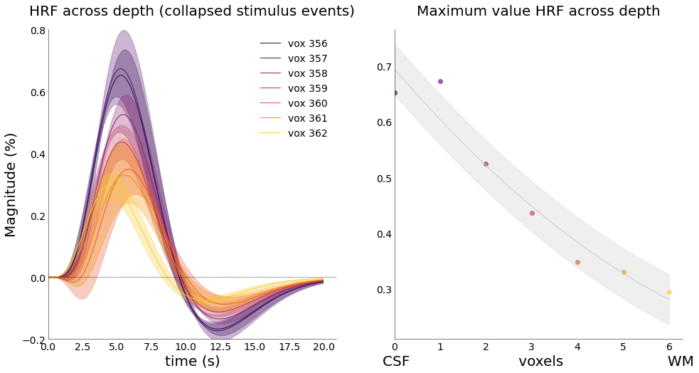
Then, we can also average across events, but not across depth. This should give use an HRF for each voxel along the cortical ribbon.
[84]:
# plot individual voxels in 1 figure
cmap = "inferno"
fig = plt.figure(figsize=(16,8))
gs = fig.add_gridspec(1,2)

ax = fig.add_subplot(gs[0])
lumped.plot_average_per_voxel(
    n_cols=None,
    figsize=(8, 8),
    axs=ax,
    font_size=font_size,
    labels=True,
    title="HRF across depth (collapsed stimulus events)",
    x_label="time (s)",
    y_label="Magnitude (%)",
    cmap=cmap,
    y_lim=[-.2,0.8])

ax = fig.add_subplot(gs[1])
lumped.plot_hrf_across_depth(
    axs=ax,
    title="Maximum value HRF across depth",
    font_size=font_size,
    cmap=cmap,
    order=2)

img = opj(func_dir, f"hrf_across_depth.png")
# fig.savefig(img, dpi=300, bbox_inches='tight')