NideconvFitter
This notebook illustrates how to perform a deconvolution using nideconv and specific classes from this repository. First, we read the data in with linescanning.dataset.Dataset, which formats our functional data and onset timings the way nideconv likes it. Then I show some useful functions to select specific portions of a larger dataframe. Then, we perform the fitting and do some plotting
[1]:
# imports
from linescanning import dataset, plotting, utils, fitting
import warnings
import os
import matplotlib.pyplot as plt
from scipy.io import loadmat
import seaborn as sns

warnings.simplefilter('ignore')
project_dir     = "/data1/projects/MicroFunc/Jurjen/projects"
base_dir        = opj(project_dir, 'hemifield')
deriv_dir       = opj(base_dir, 'derivatives')

plot_vox = 359
plot_xkcd = False
Load in some data. You could substitute this with the example data provided with the repository. However, when I did the deconvolution on that data the results didn’t look good enough for illustrative purposes. So I have a different dataset here: 3 runs of a Size-Response experiment in which our target pRF was bombarded with flickering stimuli of 5 different sizes.
[3]:
    # Load data
sub         = '003'
ses         = 3
task        = "task-SR"
runs        = [3,4,6]
func_dir    = opj(base_dir, f"sub-{sub}", f"ses-{ses}", "func")
ribbon      = (356,363)

run_files = utils.get_file_from_substring([f"sub-{sub}", f"ses-{ses}", f"{task}"], func_dir)
func_file   = utils.get_file_from_substring("bold.mat", run_files)
exp_file   = utils.get_file_from_substring("events.tsv", run_files)
func_file
[3]:
['/data1/projects/MicroFunc/Jurjen/projects/hemifield/sub-003/ses-3/func/sub-003_ses-3_task-SR_run-3_bold.mat',
 '/data1/projects/MicroFunc/Jurjen/projects/hemifield/sub-003/ses-3/func/sub-003_ses-3_task-SR_run-4_bold.mat',
 '/data1/projects/MicroFunc/Jurjen/projects/hemifield/sub-003/ses-3/func/sub-003_ses-3_task-SR_run-6_bold.mat']
Here we plop everything in Dataset, which will automatically format the functional data and onset timings for us
[4]:
window = 19
order = 3

## window 5 TR poly 2
data_obj = dataset.Dataset(
    func_file,
    deleted_first_timepoints=50,
    deleted_last_timepoints=50,
    tsv_file=exp_file,
    standardization="psc",
    use_bids=True,
    verbose=True)

df_func     = data_obj.fetch_fmri()
df_onsets   = data_obj.fetch_onsets()
df_func
DATASET

FUNCTIONAL
Preprocessing /data1/projects/MicroFunc/Jurjen/projects/hemifield/sub-003/ses-3/func/sub-003_ses-3_task-SR_run-3_bold.mat
 Filtering strategy: 'hp'
 Standardization strategy: 'psc'
 Baseline is 20 seconds, or 190 TRs
 Cutting 50 volumes from beginning (also cut from baseline (was 190, now 140 TRs) | 50 volumes from end
 DCT-high pass filter [removes low frequencies <0.01 Hz] to correct low-frequency drifts.
 tSNR [no cleaning]: 18.57      | variance: 0.76
Preprocessing /data1/projects/MicroFunc/Jurjen/projects/hemifield/sub-003/ses-3/func/sub-003_ses-3_task-SR_run-4_bold.mat
 Filtering strategy: 'hp'
 Standardization strategy: 'psc'
 Baseline is 20 seconds, or 190 TRs
 Cutting 50 volumes from beginning (also cut from baseline (was 190, now 140 TRs) | 50 volumes from end
 DCT-high pass filter [removes low frequencies <0.01 Hz] to correct low-frequency drifts.
 tSNR [no cleaning]: 19.9       | variance: 0.7
Preprocessing /data1/projects/MicroFunc/Jurjen/projects/hemifield/sub-003/ses-3/func/sub-003_ses-3_task-SR_run-6_bold.mat
 Filtering strategy: 'hp'
 Standardization strategy: 'psc'
 Baseline is 20 seconds, or 190 TRs
 Cutting 50 volumes from beginning (also cut from baseline (was 190, now 140 TRs) | 50 volumes from end
 DCT-high pass filter [removes low frequencies <0.01 Hz] to correct low-frequency drifts.
 tSNR [no cleaning]: 22.81      | variance: 0.51

EXPTOOLS
Preprocessing /data1/projects/MicroFunc/Jurjen/projects/hemifield/sub-003/ses-3/func/sub-003_ses-3_task-SR_run-3_events.tsv
 1st 't' @153.63s
 Cutting 158.88s from onsets
Preprocessing /data1/projects/MicroFunc/Jurjen/projects/hemifield/sub-003/ses-3/func/sub-003_ses-3_task-SR_run-4_events.tsv
 1st 't' @109.93s
 Cutting 115.18s from onsets
Preprocessing /data1/projects/MicroFunc/Jurjen/projects/hemifield/sub-003/ses-3/func/sub-003_ses-3_task-SR_run-6_events.tsv
 1st 't' @117.54s
 Cutting 122.79s from onsets

DATASET: created
Fetching dataframe from attribute 'df_func_psc'
[4]:
| vox 0 | vox 1 | vox 2 | vox 3 | vox 4 | vox 5 | vox 6 | vox 7 | vox 8 | vox 9 | ... | vox 710 | vox 711 | vox 712 | vox 713 | vox 714 | vox 715 | vox 716 | vox 717 | vox 718 | vox 719 | |||
|---|---|---|---|---|---|---|---|---|---|---|---|---|---|---|---|---|---|---|---|---|---|---|---|
| subject | run | t | |||||||||||||||||||||
| 003 | 3 | 0.000 | -12.112968 | 19.506470 | 2.824623 | 4.858002 | 18.645103 | -2.485558 | -6.216919 | 7.644806 | 0.117371 | 6.472908 | ... | -6.598740 | 1.931831 | -24.877098 | 10.088448 | 19.764313 | 36.417015 | -5.627525 | -36.341358 | -37.167282 | 8.782722 |
| 0.105 | 4.666885 | 2.531631 | 1.025208 | -18.671684 | 10.393379 | 12.552147 | 0.722404 | 3.682724 | -8.450172 | -1.327126 | ... | 36.637909 | -0.559746 | 55.097725 | 65.572563 | 25.778519 | -17.483330 | 42.961082 | 45.405258 | -24.064095 | -20.184967 | ||
| 0.210 | 16.257484 | 4.003906 | -9.382889 | 13.984055 | 2.706932 | 13.688568 | 1.906990 | -9.894966 | 8.269630 | -4.537666 | ... | 17.508385 | -38.955162 | -25.645264 | 20.689186 | 26.801971 | -31.645752 | -14.109596 | -7.489403 | -84.622162 | 16.263290 | ||
| 0.315 | 0.886009 | 2.582954 | 10.709297 | 11.684601 | 3.227837 | 17.266602 | 15.199478 | 3.357285 | -1.714493 | 8.968109 | ... | -20.445503 | 30.488655 | -2.957588 | -12.083633 | 8.490105 | -1.388046 | 28.978462 | 37.057465 | -32.214935 | 7.495415 | ||
| 0.420 | -0.394203 | -12.422836 | -4.406075 | 20.674042 | -3.449020 | 4.288391 | 2.411728 | 0.899651 | 10.229424 | 5.472664 | ... | 14.946091 | 1.035431 | -41.714191 | -0.333504 | 32.325989 | -21.178391 | 12.479088 | -46.943787 | -35.050156 | -22.763206 | ||
| ... | ... | ... | ... | ... | ... | ... | ... | ... | ... | ... | ... | ... | ... | ... | ... | ... | ... | ... | ... | ... | ... | ... | |
| 6 | 450.975 | -16.968468 | -1.933022 | -3.851868 | 2.879868 | -1.720558 | 2.782768 | 5.106194 | -6.267616 | 9.162407 | -2.001717 | ... | -21.017609 | -2.732735 | 3.540390 | 7.482758 | 4.214661 | 7.507225 | 55.524872 | 14.318832 | 6.575912 | 18.710037 | |
| 451.080 | 6.370689 | 15.884895 | 0.679214 | -5.673798 | 5.454056 | 2.877632 | -0.669907 | 4.443268 | 5.889519 | 7.889275 | ... | -20.272133 | -3.153091 | 17.593964 | -12.577377 | 11.167923 | 19.854065 | 58.259186 | -40.992596 | -17.050148 | -1.120850 | ||
| 451.185 | -8.917702 | -15.020752 | 2.017090 | -14.353874 | -6.002953 | -4.093712 | -2.435738 | -14.841270 | 1.449539 | -9.234657 | ... | -29.918221 | -12.623344 | 30.750786 | 23.410027 | 0.281418 | 3.630928 | -26.330490 | -6.517128 | -19.148064 | 16.913673 | ||
| 451.290 | -3.402466 | -2.567574 | -11.832848 | -3.837036 | -9.614151 | -3.799995 | 0.346992 | -2.144806 | -8.050407 | -7.654427 | ... | -18.555824 | -18.418892 | -9.471703 | 42.564392 | 30.646057 | -2.343399 | 35.635635 | -3.880394 | -36.661835 | 34.903862 | ||
| 451.395 | -3.352692 | -0.432274 | 12.870880 | 7.134697 | -0.377335 | 7.746712 | 1.689529 | -5.669823 | 2.193672 | -3.824074 | ... | 14.384300 | 13.308815 | -5.738548 | 39.509338 | -12.725807 | 9.444901 | -23.167389 | -51.609962 | 17.805450 | -3.894577 |
13300 rows × 720 columns
Now we have our data formatted the way nideconv likes it: the functional data is indexed by subject, run, and t, while the onset dataframe is indexed by subject, run, and event_type:
[5]:
df_func.head()
[5]:
| vox 0 | vox 1 | vox 2 | vox 3 | vox 4 | vox 5 | vox 6 | vox 7 | vox 8 | vox 9 | ... | vox 710 | vox 711 | vox 712 | vox 713 | vox 714 | vox 715 | vox 716 | vox 717 | vox 718 | vox 719 | |||
|---|---|---|---|---|---|---|---|---|---|---|---|---|---|---|---|---|---|---|---|---|---|---|---|
| subject | run | t | |||||||||||||||||||||
| 003 | 3 | 0.000 | -12.112968 | 19.506470 | 2.824623 | 4.858002 | 18.645103 | -2.485558 | -6.216919 | 7.644806 | 0.117371 | 6.472908 | ... | -6.598740 | 1.931831 | -24.877098 | 10.088448 | 19.764313 | 36.417015 | -5.627525 | -36.341358 | -37.167282 | 8.782722 |
| 0.105 | 4.666885 | 2.531631 | 1.025208 | -18.671684 | 10.393379 | 12.552147 | 0.722404 | 3.682724 | -8.450172 | -1.327126 | ... | 36.637909 | -0.559746 | 55.097725 | 65.572563 | 25.778519 | -17.483330 | 42.961082 | 45.405258 | -24.064095 | -20.184967 | ||
| 0.210 | 16.257484 | 4.003906 | -9.382889 | 13.984055 | 2.706932 | 13.688568 | 1.906990 | -9.894966 | 8.269630 | -4.537666 | ... | 17.508385 | -38.955162 | -25.645264 | 20.689186 | 26.801971 | -31.645752 | -14.109596 | -7.489403 | -84.622162 | 16.263290 | ||
| 0.315 | 0.886009 | 2.582954 | 10.709297 | 11.684601 | 3.227837 | 17.266602 | 15.199478 | 3.357285 | -1.714493 | 8.968109 | ... | -20.445503 | 30.488655 | -2.957588 | -12.083633 | 8.490105 | -1.388046 | 28.978462 | 37.057465 | -32.214935 | 7.495415 | ||
| 0.420 | -0.394203 | -12.422836 | -4.406075 | 20.674042 | -3.449020 | 4.288391 | 2.411728 | 0.899651 | 10.229424 | 5.472664 | ... | 14.946091 | 1.035431 | -41.714191 | -0.333504 | 32.325989 | -21.178391 | 12.479088 | -46.943787 | -35.050156 | -22.763206 |
5 rows × 720 columns
[6]:
df_onsets.head()
[6]:
| onset | |||
|---|---|---|---|
| subject | run | event_type | |
| 003 | 3 | 2.014613132977678 | 24.363776 |
| 3.5652478065289 | 35.213706 | ||
| 2.13914868391734 | 39.913720 | ||
| 3.5652478065289 | 47.413652 | ||
| 2.014613132977678 | 53.213640 |
Theoretically, nideconv should be able to concatenate multiple runs. Unfortunately, I haven’t been able to get this to work yet, so what you can do instead is run the fitter for separate runs and then average the results. Alternatively, you can concatenate the runs yourself, but that becomes tricky with onset times (maybe I should implement such an option in linescanning.dataset.Dataset..).
In any case, you can select portions of dataframes using utils.select_from_df given an expression. This expression is written in the form of how you say it. For instance: “I want the data of subject 1 and run 1”, you’d specify: utils.select_from_df(<dataframe>, expression=("subject = 1", "and", "run = 1")). The spaces in the expression are mandatory, as well as a separate operator in case you have multiple conditions. This is because, internally, the operator must be converted from
string to operator-function.
If your dataframe was indexed, you’ll be returned a subset of the dataframe conform your expression with the same indexing.
[7]:
# this is a bit simple because we only have 3 run in this dataset, but it illustrates the principle
utils.select_from_df(df_func, expression="run = 3")
[7]:
| vox 0 | vox 1 | vox 2 | vox 3 | vox 4 | vox 5 | vox 6 | vox 7 | vox 8 | vox 9 | ... | vox 710 | vox 711 | vox 712 | vox 713 | vox 714 | vox 715 | vox 716 | vox 717 | vox 718 | vox 719 | |||
|---|---|---|---|---|---|---|---|---|---|---|---|---|---|---|---|---|---|---|---|---|---|---|---|
| subject | run | t | |||||||||||||||||||||
| 003 | 3 | 0.000 | -12.112968 | 19.506470 | 2.824623 | 4.858002 | 18.645103 | -2.485558 | -6.216919 | 7.644806 | 0.117371 | 6.472908 | ... | -6.598740 | 1.931831 | -24.877098 | 10.088448 | 19.764313 | 36.417015 | -5.627525 | -36.341358 | -37.167282 | 8.782722 |
| 0.105 | 4.666885 | 2.531631 | 1.025208 | -18.671684 | 10.393379 | 12.552147 | 0.722404 | 3.682724 | -8.450172 | -1.327126 | ... | 36.637909 | -0.559746 | 55.097725 | 65.572563 | 25.778519 | -17.483330 | 42.961082 | 45.405258 | -24.064095 | -20.184967 | ||
| 0.210 | 16.257484 | 4.003906 | -9.382889 | 13.984055 | 2.706932 | 13.688568 | 1.906990 | -9.894966 | 8.269630 | -4.537666 | ... | 17.508385 | -38.955162 | -25.645264 | 20.689186 | 26.801971 | -31.645752 | -14.109596 | -7.489403 | -84.622162 | 16.263290 | ||
| 0.315 | 0.886009 | 2.582954 | 10.709297 | 11.684601 | 3.227837 | 17.266602 | 15.199478 | 3.357285 | -1.714493 | 8.968109 | ... | -20.445503 | 30.488655 | -2.957588 | -12.083633 | 8.490105 | -1.388046 | 28.978462 | 37.057465 | -32.214935 | 7.495415 | ||
| 0.420 | -0.394203 | -12.422836 | -4.406075 | 20.674042 | -3.449020 | 4.288391 | 2.411728 | 0.899651 | 10.229424 | 5.472664 | ... | 14.946091 | 1.035431 | -41.714191 | -0.333504 | 32.325989 | -21.178391 | 12.479088 | -46.943787 | -35.050156 | -22.763206 | ||
| ... | ... | ... | ... | ... | ... | ... | ... | ... | ... | ... | ... | ... | ... | ... | ... | ... | ... | ... | ... | ... | ... | ||
| 450.975 | 1.725731 | -15.144714 | -19.009155 | -3.102150 | 12.564888 | 2.306580 | 1.190056 | -5.206390 | 3.865814 | -11.063164 | ... | 11.005417 | 43.028572 | -13.639664 | -11.605675 | -26.643242 | 11.073257 | 34.346077 | -15.131874 | -3.783920 | 16.046173 | ||
| 451.080 | -3.356529 | 3.235062 | 6.483208 | 8.875519 | -6.379730 | -4.626564 | -13.571541 | -10.956978 | 3.768692 | -4.126717 | ... | -26.043411 | 51.461571 | 19.043587 | -24.526794 | 6.236290 | 6.885307 | -4.252258 | 4.819321 | 9.252182 | 9.920586 | ||
| 451.185 | -6.879913 | 2.792343 | -2.592278 | 0.779831 | 1.908806 | -12.933929 | 8.834854 | 6.723106 | -11.457649 | 12.841576 | ... | 19.375526 | 38.798744 | 10.708488 | -27.424278 | -26.934189 | -29.444199 | 2.804276 | 19.032402 | -25.089104 | -6.882072 | ||
| 451.290 | 5.931419 | -3.274689 | 17.510986 | 5.629753 | 0.361130 | 13.059998 | -9.553940 | 4.909546 | 1.226761 | -6.461479 | ... | -10.643494 | 22.493546 | 36.711357 | -17.700424 | -57.566364 | -13.176224 | 25.810303 | 30.254288 | 17.943405 | 16.263077 | ||
| 451.395 | -5.419510 | -1.785980 | -0.812332 | 1.738518 | 4.302994 | -0.589066 | 5.135925 | 7.422478 | -2.608772 | 5.147690 | ... | -2.996056 | 18.514374 | -2.529625 | 5.339706 | 3.317848 | -44.731350 | 17.661545 | -22.539970 | -18.592567 | 44.011917 |
4300 rows × 720 columns
We can also select only the voxels from the GM-ribbon. For convenience, we’ll continue with this subset of the dataframe for our fitting
[8]:
df_ribbon = utils.select_from_df(df_func, expression='ribbon', indices=ribbon)
df_ribbon
[8]:
| vox 356 | vox 357 | vox 358 | vox 359 | vox 360 | vox 361 | vox 362 | |||
|---|---|---|---|---|---|---|---|---|---|
| subject | run | t | |||||||
| 003 | 3 | 0.000 | -0.071739 | 0.167107 | -0.144806 | -4.456978 | -4.997894 | -8.061729 | -6.211449 |
| 0.105 | -2.024399 | -3.539673 | -1.894897 | -1.422615 | -0.659103 | -0.154816 | 1.179634 | ||
| 0.210 | -1.272415 | 0.316490 | 1.884216 | 0.062370 | -3.012459 | -2.817741 | -1.851486 | ||
| 0.315 | 1.462990 | 1.300804 | 3.058662 | -0.195541 | 2.700043 | -0.468964 | 2.553284 | ||
| 0.420 | 2.638489 | 3.550682 | 1.020058 | 3.021248 | -0.796242 | 0.847038 | -2.357117 | ||
| ... | ... | ... | ... | ... | ... | ... | ... | ... | |
| 6 | 450.975 | 1.175598 | 3.093842 | 0.262177 | 1.514366 | -0.397339 | 3.008080 | 1.352455 | |
| 451.080 | 4.563950 | 0.574020 | 3.470749 | 2.962746 | 3.178062 | 1.342949 | 0.326973 | ||
| 451.185 | -2.680687 | 1.237396 | 0.730515 | -0.935905 | -0.360039 | 2.012772 | -0.274796 | ||
| 451.290 | 3.334953 | -1.183098 | 0.452560 | 1.486267 | 1.584473 | -1.043343 | 0.097862 | ||
| 451.395 | -1.214912 | -1.032112 | 0.330559 | -0.220901 | 1.206627 | 1.044044 | 0.799171 |
13300 rows × 7 columns
[9]:
# this also works for onset dataframes
utils.select_from_df(df_onsets, expression="run = 3")
[9]:
| onset | |||
|---|---|---|---|
| subject | run | event_type | |
| 003 | 3 | 2.014613132977678 | 24.363776 |
| 3.5652478065289 | 35.213706 | ||
| 2.13914868391734 | 39.913720 | ||
| 3.5652478065289 | 47.413652 | ||
| 2.014613132977678 | 53.213640 | ||
| 3.5652478065289 | 60.755378 | ||
| 1.853928859395028 | 65.730180 | ||
| 1.853928859395028 | 78.388490 | ||
| 3.5652478065289 | 91.713437 | ||
| 1.140879298089248 | 101.380051 | ||
| 1.140879298089248 | 107.305134 | ||
| 1.853928859395028 | 113.854985 | ||
| 1.853928859395028 | 118.821583 | ||
| 1.140879298089248 | 124.246617 | ||
| 2.014613132977678 | 134.221550 | ||
| 2.13914868391734 | 143.271515 | ||
| 3.5652478065289 | 148.613325 | ||
| 1.140879298089248 | 156.696457 | ||
| 3.5652478065289 | 165.754301 | ||
| 1.140879298089248 | 173.188099 | ||
| 2.13914868391734 | 177.813011 | ||
| 2.014613132977678 | 183.387938 | ||
| 1.140879298089248 | 189.746253 | ||
| 1.140879298089248 | 197.829608 | ||
| 2.014613132977678 | 203.704453 | ||
| 2.13914868391734 | 209.404494 | ||
| 3.5652478065289 | 214.246153 | ||
| 3.5652478065289 | 219.679502 | ||
| 1.853928859395028 | 229.487711 | ||
| 1.853928859395028 | 236.129379 | ||
| 2.13914868391734 | 253.129303 | ||
| 1.853928859395028 | 263.112592 | ||
| 1.853928859395028 | 269.629237 | ||
| 2.13914868391734 | 274.529287 | ||
| 2.13914868391734 | 280.462811 | ||
| 2.014613132977678 | 285.129148 | ||
| 1.853928859395028 | 291.412421 | ||
| 2.014613132977678 | 300.354080 | ||
| 2.014613132977678 | 306.204038 | ||
| 2.014613132977678 | 314.637343 | ||
| 2.014613132977678 | 320.537317 | ||
| 1.140879298089248 | 333.486816 | ||
| 1.140879298089248 | 344.870505 | ||
| 1.140879298089248 | 354.812066 | ||
| 1.853928859395028 | 360.437064 | ||
| 3.5652478065289 | 365.712135 | ||
| 3.5652478065289 | 370.870303 | ||
| 2.13914868391734 | 376.503695 | ||
| 2.13914868391734 | 386.603704 | ||
| 2.13914868391734 | 392.345201 |
Right, on to the fitting: we can do the fitting with utils.NideconvFitter, which requires the functional dataframe, onset dataframe, and some settings on the type of fit you’d like to do, number of regressors, confounds, etc
[299]:
nd_fit = fitting.NideconvFitter(
    df_ribbon,
    df_onsets,
    basis_sets='canonical_hrf_with_time_derivative',
    lump_events=False,
    TR=0.105,
    interval=[-3,17],
    add_intercept=True,
    verbose=True,
    fit=True)

nd_fit.timecourses_condition()
Selected 'canonical_hrf_with_time_derivative'-basis sets
Adding event '1.140879298089248' to model
Adding event '1.853928859395028' to model
Adding event '2.014613132977678' to model
Adding event '2.13914868391734' to model
Adding event '3.5652478065289' to model
Fitting with 'ols' minimization
Done
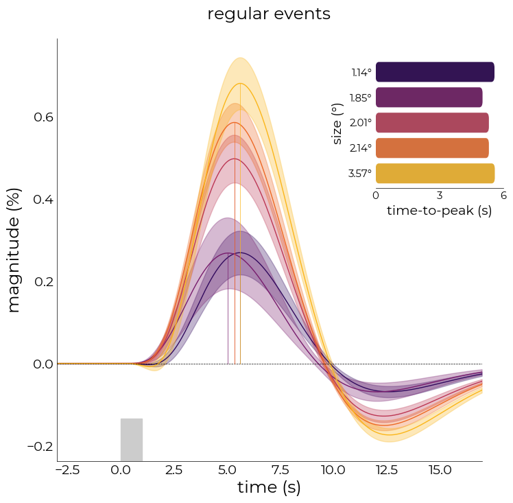
With plot_average_per_event, we can plot the average response across the voxels in the dataframe for each event in the model. We can also prettify the figure by adding an inset containing the time-to-peak barplot
[286]:
%matplotlib inline
fig,axs = plt.subplots(figsize=(8,8))
nd_fit.plot_average_per_event(
    xkcd=plot_xkcd,
    x_label="time (s)",
    y_label="magnitude (%)",
    add_hline='default',
    axs=axs,
    ttp=True,
    lim=[0, 6],
    ticks=[0, 3, 6],
    ttp_lines=True,
    y_label2="size (°)",
    x_label2="time-to-peak (s)",
    title="regular events",
    ttp_labels=[f"{round(float(ii),2)}°" for ii in nd_fit.cond],
    add_labels=True,
    fancy=True,
    cmap='inferno')

# plot stimulus onset
axs.axvspan(0,1, ymax=0.1, color="#cccccc")
[286]:
<matplotlib.patches.Polygon at 0x7fd2ddbdd2b0>
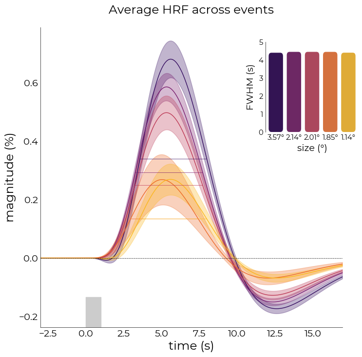
Or full-with half maximum (FWHM)
[288]:
fig,axs = plt.subplots(figsize=(8,8))
nd_fit.plot_average_per_event(
    x_label="time (s)",
    y_label="magnitude (%)",
    add_hline='default',
    axs=axs,
    fwhm=True,
    fwhm_lines=True,
    lim=[0,5],
    ticks=[i for i in range(6)],
    fwhm_labels=[f"{round(float(ii),2)}°" for ii in nd_fit.cond[::-1]],
    events=nd_fit.cond[::-1],
    add_labels=True,
    x_label2="size (°)",
    y_label2="FWHM (s)",
    fancy=True,
    cmap='inferno')

# plot stimulus onset
axs.axvspan(0,1, ymax=0.1, color="#cccccc")
Flipping events to ['3.5652478065289' '2.13914868391734' '2.014613132977678'
 '1.853928859395028' '1.140879298089248']
[288]:
<matplotlib.patches.Polygon at 0x7fd2ddc2beb0>
[300]:
# individual model fits
fit_objs = []
for ii in nd_fit.cond:

    nd_ = fitting.NideconvFitter(
        df_ribbon,
        utils.select_from_df(df_onsets, expression=f"event_type = {ii}"),
        basis_sets='canonical_hrf_with_time_derivative',
        TR=0.105,
        interval=[-3,18],
        add_intercept=True,
        verbose=True)

    nd_.timecourses_condition()
    fit_objs.append(nd_)
Selected 'canonical_hrf_with_time_derivative'-basis sets
Adding event '1.140879298089248' to model
Fitting with 'ols' minimization
Done
Selected 'canonical_hrf_with_time_derivative'-basis sets
Adding event '1.853928859395028' to model
Fitting with 'ols' minimization
Done
Selected 'canonical_hrf_with_time_derivative'-basis sets
Adding event '2.014613132977678' to model
Fitting with 'ols' minimization
Done
Selected 'canonical_hrf_with_time_derivative'-basis sets
Adding event '2.13914868391734' to model
Fitting with 'ols' minimization
Done
Selected 'canonical_hrf_with_time_derivative'-basis sets
Adding event '3.5652478065289' to model
Fitting with 'ols' minimization
Done
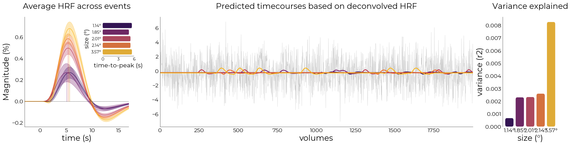
[310]:
from sklearn.metrics import r2_score

fig = plt.figure(figsize=(24,5))
gs = fig.add_gridspec(1,3, width_ratios=[1,3,0.5], wspace=0.2)
font_size = 20

ax1 = fig.add_subplot(gs[0])
nd_fit.plot_average_per_event(
    axs=ax1,
    x_label="time (s)",
    y_label="Magnitude (%)",
    add_hline='default',
    ttp=True,
    ttp_lines=True,
    add_labels=True,
    y_label2="size (°)",
    x_label2="time-to-peak (s)",
    ttp_labels=[f"{round(float(ii),2)}°" for ii in nd_fit.cond],
    lim=[0, 6],
    ticks=[0,3,6],
    cmap='inferno',
    fancy=True,
    font_size=font_size)

ax2 = fig.add_subplot(gs[1])
colors = sns.color_palette('inferno', len(nd_fit.cond))
preds = [utils.select_from_df(fit_objs[ii].predictions, expression="run = 3").iloc[:,0].values for ii in range(len(fit_objs))]
real = utils.select_from_df(df_ribbon, expression="run = 3").iloc[:, 0].values

plotting.LazyPlot(
    [ii[:2000] for ii in [real]+preds],
    line_width=[0.5]+[2 for ii in range(len(fit_objs))],
    color=["#cccccc"]+colors,
    axs=ax2,
    title="Predicted timecourses based on deconvolved HRF",
    font_size=font_size,
    x_label="volumes")

# calculate r2's
ax3 = fig.add_subplot(gs[2])
r2s = [r2_score(real, preds[ii]) for ii in range(len(fit_objs))]
plotting.LazyBar(
    x=[f"{round(float(ii),2)}°" for ii in nd_fit.cond],
    y=r2s,
    palette=colors,
    sns_ori="v",
    axs=ax3,
    add_labels=True,
    x_label2="size (°)",
    y_label2="variance (r2)",
    font_size=font_size,
    title2="Variance explained",
    fancy_denom=8,
    sns_offset=4,
    fancy=True)
[310]:
<linescanning.plotting.LazyBar at 0x7fd2dbd56a00>
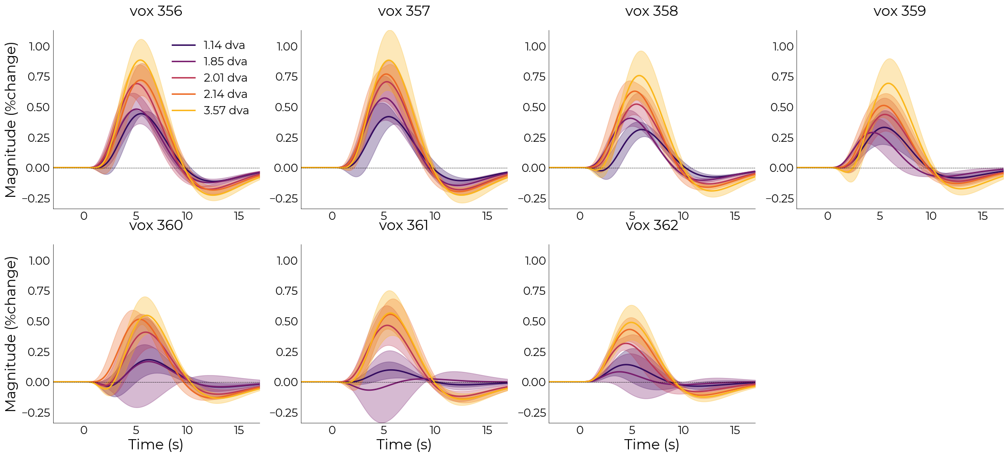
[314]:
nd_fit.plot_average_per_voxel(
    labels=[f"{round(float(ii),2)} dva" for ii in nd_fit.cond],
    wspace=0.2,
    cmap="inferno",
    line_width=2,
    font_size=font_size,
    label_size=16,
    sharey=True)
    # save_as=opj(func_dir, "hrf_gamma_voxel.png"))
Above, we defined each stimulus size as separate event. To investigate a global response, we can also lump all the events together using lump_events=True. This means we’ll interpret any event as 1 event:
[289]:
lumped = fitting.NideconvFitter(
    df_ribbon,
    df_onsets,
    confounds=None,
    basis_sets='fourier',
    n_regressors=4,
    lump_events=True,
    TR=0.105,
    interval=[-3,17],
    add_intercept=True,
    verbose=True)
Selected 'fourier'-basis sets
Adding event 'stim' to model
Fitting with 'ols' minimization
Done
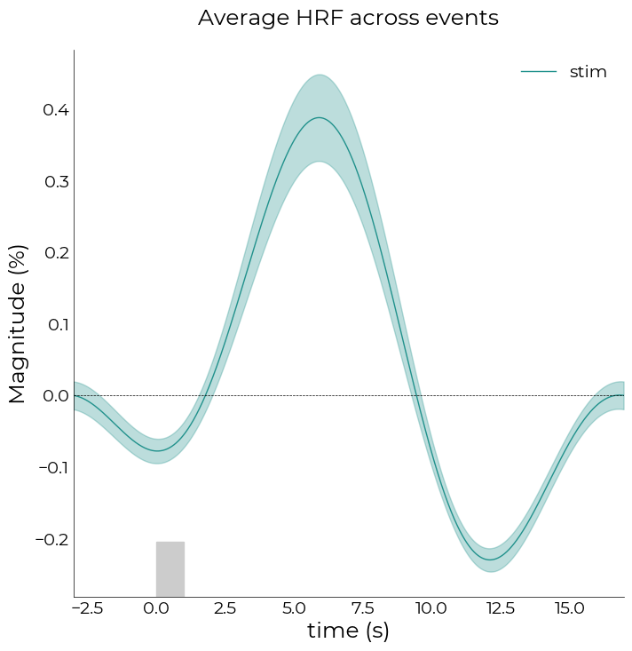
[293]:
# plot average across voxels
fig,axs = plt.subplots(figsize=(8,8))
lumped.plot_average_per_event(
    labels=['stim'],
    figsize=(8,8),
    axs=axs,
    x_label="time (s)",
    y_label="Magnitude (%)",
    add_hline='default')

# plot stimulus onset
axs.axvspan(0,1, ymax=0.1, color="#cccccc")
[293]:
<matplotlib.patches.Polygon at 0x7fd2dec97d30>
[294]:
lumped.tc_condition
[294]:
| vox 356 | vox 357 | vox 358 | vox 359 | vox 360 | vox 361 | vox 362 | |||
|---|---|---|---|---|---|---|---|---|---|
| event_type | covariate | time | |||||||
| stim | intercept | -3.00000 | -0.092421 | -0.062954 | -0.027623 | -0.010078 | 0.039126 | 0.049183 | 0.003650 |
| -2.99475 | -0.092423 | -0.063035 | -0.027751 | -0.010080 | 0.039143 | 0.049162 | 0.003655 | ||
| -2.98950 | -0.092427 | -0.063118 | -0.027881 | -0.010082 | 0.039158 | 0.049140 | 0.003659 | ||
| -2.98425 | -0.092431 | -0.063201 | -0.028011 | -0.010086 | 0.039172 | 0.049117 | 0.003663 | ||
| -2.97900 | -0.092435 | -0.063285 | -0.028142 | -0.010091 | 0.039184 | 0.049093 | 0.003667 | ||
| ... | ... | ... | ... | ... | ... | ... | ... | ||
| 16.92375 | -0.092418 | -0.062640 | -0.027123 | -0.010085 | 0.039045 | 0.049252 | 0.003625 | ||
| 16.92900 | -0.092418 | -0.062717 | -0.027247 | -0.010081 | 0.039067 | 0.049237 | 0.003632 | ||
| 16.93425 | -0.092418 | -0.062795 | -0.027371 | -0.010079 | 0.039088 | 0.049220 | 0.003638 | ||
| 16.93950 | -0.092419 | -0.062874 | -0.027497 | -0.010078 | 0.039108 | 0.049202 | 0.003644 | ||
| 16.94475 | -0.092421 | -0.062954 | -0.027623 | -0.010078 | 0.039126 | 0.049183 | 0.003650 |
3800 rows × 7 columns
[295]:
# plot individual voxels in separete figures
lumped.plot_average_per_voxel(
    labels=['stim'],
    n_cols=7,
    figsize=(40,5),
    wspace=0.3)

With this lumped-event model, we can also plot the HRFs across depth, independent of stimulus size (left plot). We can then extract the maximums of all HRFs and fit a polynomial to it, revealing a trend towards decreased HRF-amplitude when going from CSF/GM to GM/WM borders
[322]:
# plot individual voxels in 1 figure
fig = plt.figure(figsize=(16, 8))
gs = fig.add_gridspec(1, 2)

ax = fig.add_subplot(gs[0])
lumped.plot_average_per_voxel(
    n_cols=None,
    axs=ax,
    labels=True,
    x_label="time (s)",
    y_label="Magnitude (z-score)",
    set_xlim_zero=False)
ax.set_title("HRF across depth (collapsed stimulus events)", fontsize=lumped.pl.font_size)

ax = fig.add_subplot(gs[1])
lumped.plot_hrf_across_depth(
    axs=ax,
    order=1,
    x_label="depth [%]")
ax.set_title("Maximum value HRF across depth", fontsize=lumped.pl.font_size)
[322]:
Text(0.5, 1.0, 'Maximum value HRF across depth')

[ ]: