LazyPlot 

Sometimes it’s a bit cumbersome to go through all matplotlib motions such as intiating the figure, adding labels, and such when you just want to quickly visualize your data. This class is intended to do just that. Make the same plots in a whole lot less lines. I tried to include as many functionalities as possible without overcomplicating the process too much. Below are a few examples of how to use this class.

[1]:

%reload_ext autoreload
%autoreload 2

[2]:

# imports
from linescanning import plotting, utils
import warnings
import os
import matplotlib.pyplot as plt
import seaborn as sns
import numpy as np

warnings.simplefilter('ignore')
opj = os.path.join

Create random timeseries with linescanning.utils.random_timeseries

[3]:

print(utils.random_timeseries.__doc__)

random_timeseries

    Create a random timecourse by multiplying an intercept with a random Gaussian distribution.

    Parameters
    ----------
    intercept: float
        starting point of timecourse
    volatility: float
        this factor is multiplied with the Gaussian distribution before multiplied with the intercept
    nr: int
        length of timecourse

    Returns
    ----------
    numpy.ndarray
        array of length `nr`

    Example
    ----------
    >>> from linescanning import utils
    >>> ts = utils.random_timeseries(1.2, 0.5, 100)

    Notes
    ----------
    Source: https://stackoverflow.com/questions/67977231/how-to-generate-random-time-series-data-with-noise-in-python-3

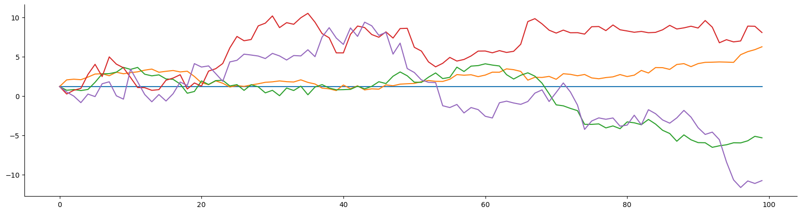
Plot them regularly

[5]:

ts = utils.random_timeseries(1.2, 0.0, 100)
ts1 = utils.random_timeseries(1.2, 0.3, 100)
ts2 = utils.random_timeseries(1.2, 0.5, 100)
ts3 = utils.random_timeseries(1.2, 0.8, 100)
ts4 = utils.random_timeseries(1.2, 1, 100)
print(ts.shape)

fig,axs = plt.subplots(figsize=(20,5))
axs.plot(ts)
axs.plot(ts1)
axs.plot(ts2)
axs.plot(ts3)
axs.plot(ts4)
sns.despine(offset=0)

(100,)

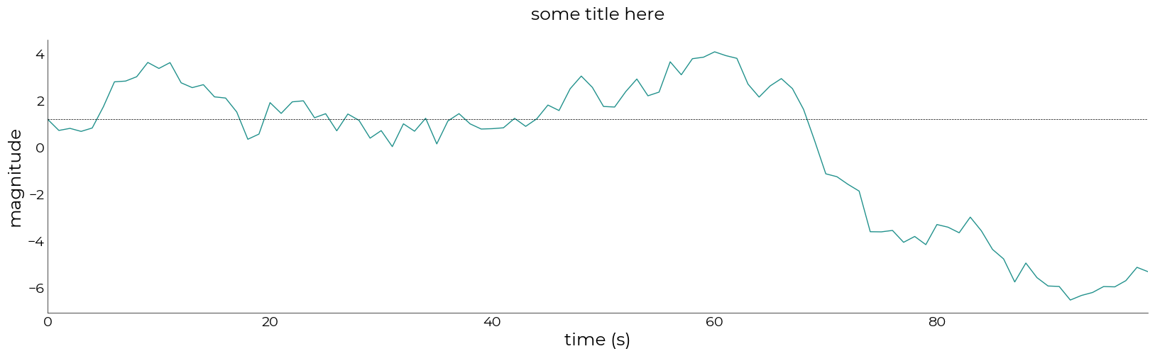
Use LazyPlot to plot a single timeseries

[15]:

plotting.LazyPlot(
    ts2,
    figsize=(20, 5),
    x_label="time (s)",
    y_label="magnitude",
    title="some title here")

[15]:

<linescanning.plotting.LazyPlot at 0x7f0315dd8820>

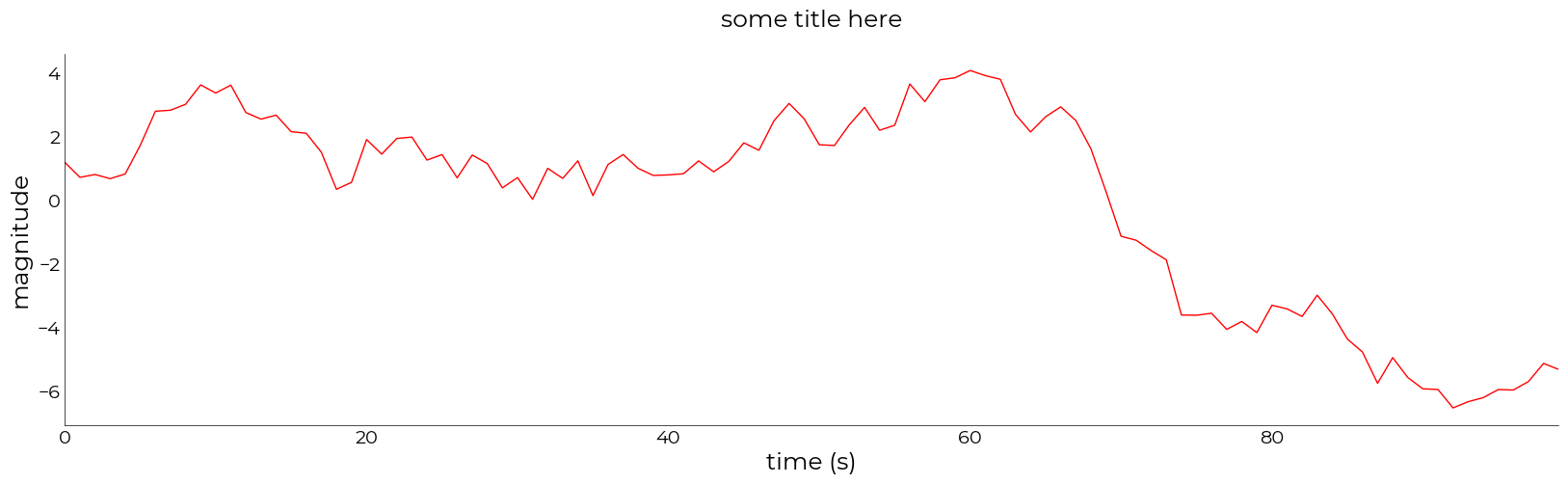
[23]:

# change the color
plotting.LazyPlot(
    ts2,
    figsize=(20, 5),
    color="r",
    x_label="time (s)",
    y_label="magnitude",
    title="some title here")

[23]:

<linescanning.plotting.LazyPlot at 0x7f030fe21f10>

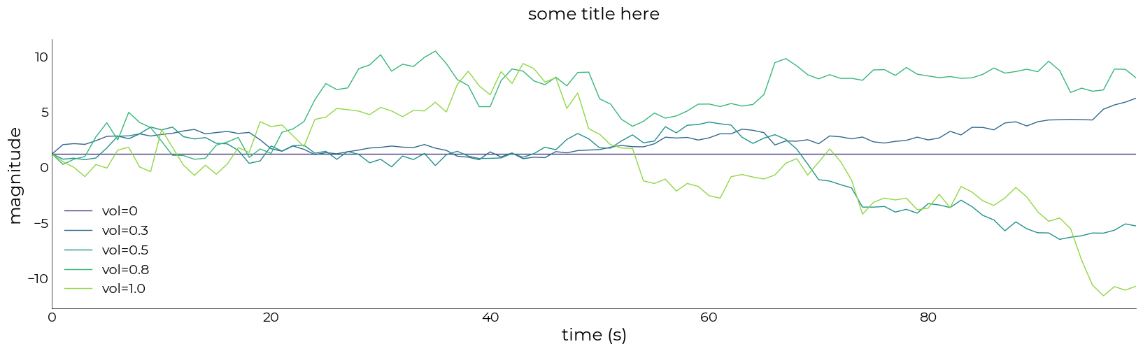
Use LazyPlot to plot multiply timeseries

[16]:

plotting.LazyPlot(
    [ts, ts1, ts2, ts3, ts4],
    figsize=(20, 5),
    # save_as="/mnt/d/FSL/shared/spinoza/programs/project_repos/PlayGround/results/test_LazyPlot.pdf",
    labels=['vol=0', 'vol=0.3', 'vol=0.5', 'vol=0.8', 'vol=1.0'],
    x_label="time (s)",
    y_label="magnitude",
    title="some title here")

[16]:

<linescanning.plotting.LazyPlot at 0x7f031592f640>

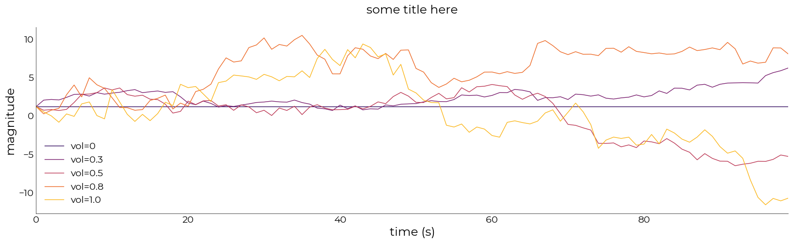
[22]:

# change colormap
plotting.LazyPlot(
    [ts, ts1, ts2, ts3, ts4],
    figsize=(20, 5),
    # save_as="/mnt/d/FSL/shared/spinoza/programs/project_repos/PlayGround/results/test_LazyPlot.pdf",
    labels=['vol=0', 'vol=0.3', 'vol=0.5', 'vol=0.8', 'vol=1.0'],
    x_label="time (s)",
    y_label="magnitude",
    title="some title here",
    cmap="inferno")

[22]:

<linescanning.plotting.LazyPlot at 0x7f0315bb34f0>

Add horizontal line

[17]:

hline = {'pos': 1.2}
plotting.LazyPlot(
    ts2,
    figsize=(20, 5),
    add_hline=hline,
    x_label="time (s)",
    y_label="magnitude",
    title="some title here")

[17]:

<linescanning.plotting.LazyPlot at 0x7f031e190f70>

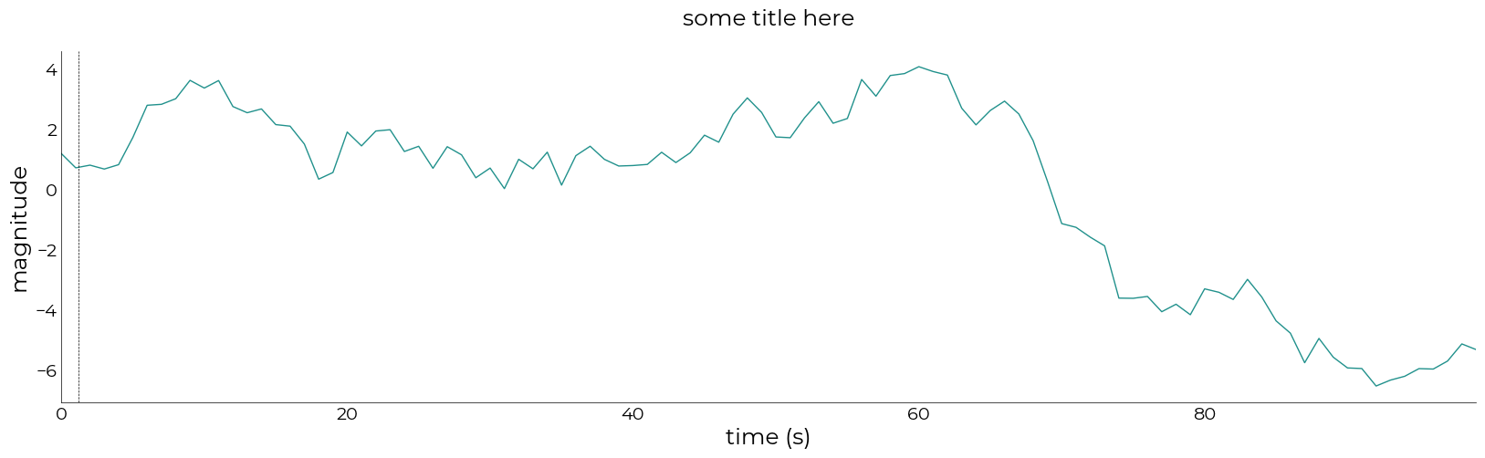
Add vertical line

[18]:

vline = {'pos': 1.2}
plotting.LazyPlot(
    ts2,
    figsize=(20, 5),
    add_vline=vline,
    x_label="time (s)",
    y_label="magnitude",
    title="some title here")

[18]:

<linescanning.plotting.LazyPlot at 0x7f03159bb640>

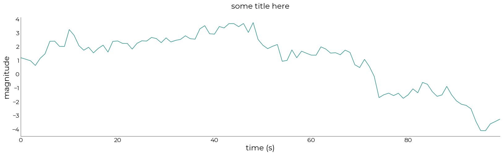
Add shaded error

[19]:

from scipy.stats import sem
stack = np.hstack((ts1[...,np.newaxis],ts2[...,np.newaxis],ts4[...,np.newaxis]))
avg = stack.mean(axis=-1)
err = sem(stack, axis=-1)
plotting.LazyPlot(
    avg,
    figsize=(20, 5),
    error=err,
    x_label="time (s)",
    y_label="magnitude",
    title="some title here")

[19]:

<linescanning.plotting.LazyPlot at 0x7f0315d1a6d0>

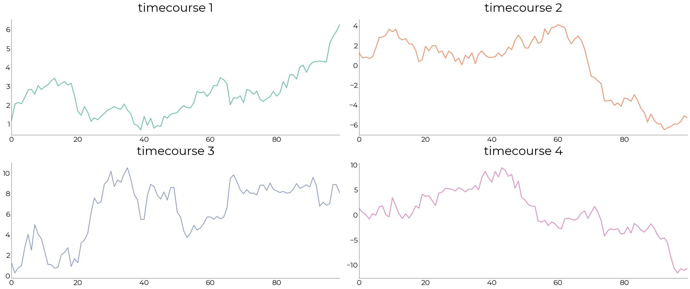
Subplotting with gridspec

[28]:

# initialize the figure. Figsize only specified in plt.figure, not in LazyPlot
fig = plt.figure(constrained_layout=True, figsize=(24,10))
# specify the grid
gs = fig.add_gridspec(2,2)

# collect fake timecourses in list so we can index them
timecourses = [ts1, ts2, ts3, ts4]
colors = sns.color_palette("Set2", len(timecourses))

for ii in range(len(timecourses)):

    # add subplot to figure on axis in gridspec
    ax = fig.add_subplot(gs[ii])

    # give the axis to LazyPlot
    plotting.LazyPlot(
        timecourses[ii],
        axs=ax,
        set_xlim_zero=True,
        title=f"timecourse {ii+1}",
        line_width=2,
        color=colors[ii],
        font_size=30,
        label_size=18)

[ ]:

LazyPlot

LazyPlot 