GenericGLM
This page shows how to implement a simple GLM using the functions embedded in linescanning.glm. First, I show how to set up the GLM using the individual functions, which is way too annoying to remember everytime you want to run a glm. For that reason, there’s also the GenericGLM class, which does everything the individual functions do but then in 1 line of code. Saves some time:). The experiment used in this example was a hemifield-stimulation experiment, so our event conditions are
‘left’ and ‘right’.
[1]:
%reload_ext autoreload
%autoreload 2
[7]:
# imports
from linescanning import glm, utils, dataset, plotting
import warnings
import os
import matplotlib.pyplot as plt
import seaborn as sns

warnings.simplefilter('ignore')
opj = os.path.join
[8]:
# define files
data_path = os.path.dirname(os.path.dirname(glm.__file__))
func_file = opj(data_path, 'examples', 'bold.mat')
exp_file = opj(data_path, 'examples', 'events.tsv')

plot_vox = 359
[48]:
# load in functional data
window = 19
order = 3
data = dataset.Dataset(func_file,
subject=1,
run=1,
deleted_first_timepoints=100,
deleted_last_timepoints=0,
window_size=window,
high_pass=True,
poly_order=order,
tsv_file=exp_file,
use_bids=False)
# fetch percent signal change
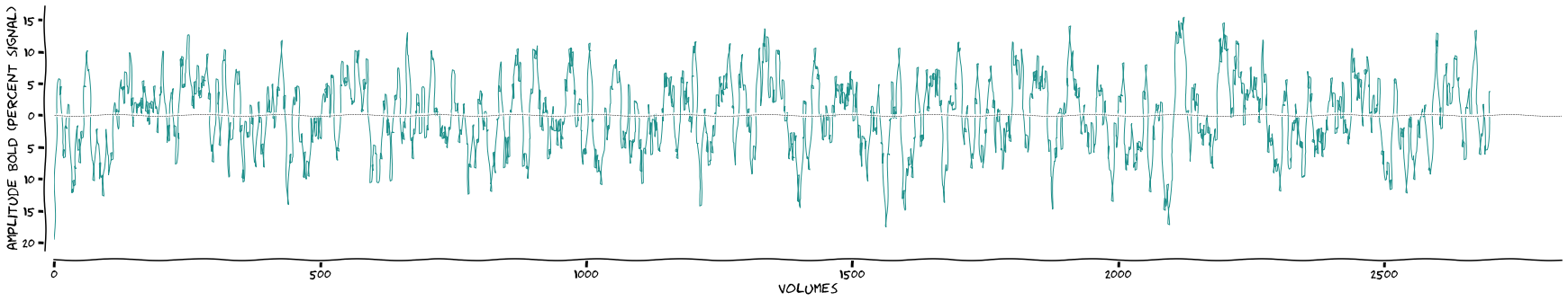
func = data.fetch_fmri(strip_index=True) # > strip the dataframe from subject, run, t indices
print(func.shape)
# plot a timecourse
plotting.LazyPlot(func.values[:,plot_vox],
font_size=16,
set_xlim_zero=True,
sns_trim=False,
add_hline='default',
x_label="volumes",
y_label="amplitude BOLD (percent signal)",
xkcd=True)
(2700, 720)
[48]:
<linescanning.plotting.LazyPlot at 0x7f77774bd130>
Onset file is already read in by Dataset via ParseExpToolsFile; onset times have been corrected for deleted volumes
[17]:
onsets = data.fetch_onsets()
onsets
[17]:
| onset | event_type | subject | run | |
|---|---|---|---|---|
| 0 | 27.961789 | right | 1 | 1 |
| 1 | 32.903438 | right | 1 | 1 |
| 2 | 37.036976 | right | 1 | 1 |
| 3 | 38.811892 | right | 1 | 1 |
| 4 | 43.937109 | right | 1 | 1 |
| ... | ... | ... | ... | ... |
| 74 | 282.608184 | right | 1 | 1 |
| 75 | 286.016544 | left | 1 | 1 |
| 76 | 289.266474 | left | 1 | 1 |
| 77 | 292.133307 | right | 1 | 1 |
| 78 | 294.224900 | right | 1 | 1 |
79 rows × 4 columns
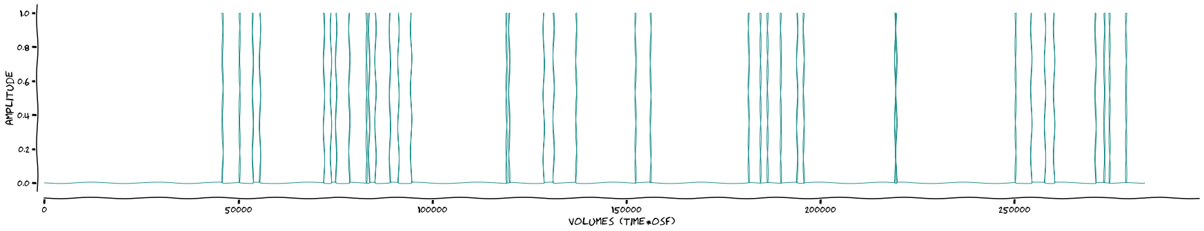
Oversample with factor 1000 to get rid of 3 decimals in onset times. The larger this factor, the more accurate decimal onset times will be processed, but also the bigger your upsampled convolved becomes, which means convolving will take longer.
[23]:
osf = 1000

# make stimulus vectors
stims = glm.make_stimulus_vector(onsets, scan_length=func.shape[0], osf=osf, type='event')
plotting.LazyPlot(stims['left'],
                  font_size=16,
                  x_label="volumes (time*osf)",
                  set_xlim_zero=True,
                  sns_trim=False,
                  y_label="amplitude",
                  xkcd=True)
stims
[23]:
{'left': array([0., 0., 0., ..., 0., 0., 0.]),
 'right': array([0., 0., 0., ..., 0., 0., 0.])}
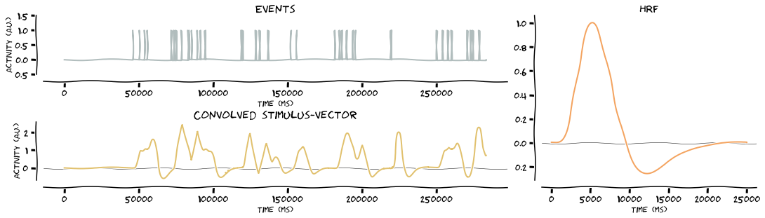
[25]:
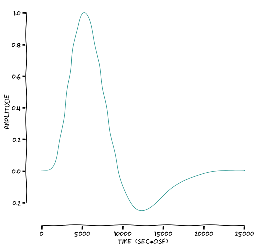
# define HRF
dt = 1/osf
time_points = np.linspace(0, 25, np.rint(float(25)/dt).astype(int))
hrf = glm.double_gamma(time_points, lag=6)
plotting.LazyPlot(hrf,
                  figsize=(8,8),
                  font_size=14,
                  x_label="time (sec*osf)",
                  y_label="amplitude",
                  xkcd=True)
[25]:
<linescanning.plotting.LazyPlot at 0x7f7793dc4190>
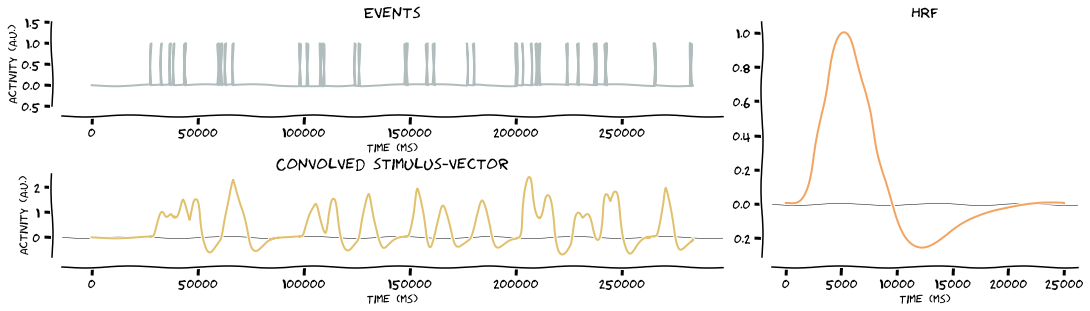
Convolve the stimulus vectors with the HRF. Because stims is a dict, the function will loop over the keys and as such, produce the outputs for all events. In this case, it’s two events, namely left stimulation and right stimulation
[26]:
# convolve stimulus vector with HRF
stim_vector = glm.convolve_hrf(hrf, stims, make_figure=True, xkcd=True)
stim_vector


[26]:
{'left': array([0.        , 0.        , 0.        , ..., 0.70500641, 0.70478048,
        0.70455449]),
 'right': array([ 0.        ,  0.        ,  0.        , ..., -0.0730913 ,
        -0.07300529, -0.07291914])}
[50]:
# resample back to time domain of functional data
stim_vector_resampled = glm.resample_stim_vector(stim_vector, func.shape[0])
stim_vector_resampled
[50]:
{'left': array([0.        , 0.        , 0.        , ..., 0.75053595, 0.72774167,
        0.70455449]),
 'right': array([ 0.        ,  0.        ,  0.        , ..., -0.0883798 ,
        -0.08117716, -0.07291914])}
[51]:
# create design matrix without regressors
design_no_regressors = glm.first_level_matrix(stim_vector_resampled)
design_no_regressors
[51]:
| intercept | left | right | |
|---|---|---|---|
| 0 | 1.0 | 0.000000 | 0.000000 |
| 1 | 1.0 | 0.000000 | 0.000000 |
| 2 | 1.0 | 0.000000 | 0.000000 |
| 3 | 1.0 | 0.000000 | 0.000000 |
| 4 | 1.0 | 0.000000 | 0.000000 |
| ... | ... | ... | ... |
| 2695 | 1.0 | 0.794522 | -0.100938 |
| 2696 | 1.0 | 0.772771 | -0.094854 |
| 2697 | 1.0 | 0.750536 | -0.088380 |
| 2698 | 1.0 | 0.727742 | -0.081177 |
| 2699 | 1.0 | 0.704554 | -0.072919 |
2700 rows × 3 columns
[52]:
# create some fake regressors
regressors = np.zeros((func.shape[0],5))
for ii in range(regressors.shape[-1]):
    regressors[...,ii] = utils.random_timeseries(1.2,(ii/8),func.shape[0])
[53]:
# create design matrix with regressors
design_regressors = glm.first_level_matrix(stim_vector_resampled, regressors=regressors)
design_regressors
[53]:
| intercept | left | right | regressor 0 | regressor 1 | regressor 2 | regressor 3 | regressor 4 | |
|---|---|---|---|---|---|---|---|---|
| 0 | 1.0 | 0.000000 | 0.000000 | 1.2 | 1.200000 | 1.200000 | 1.200000 | 1.200000 |
| 1 | 1.0 | 0.000000 | 0.000000 | 1.2 | 1.085555 | 1.050038 | 0.235860 | 1.557244 |
| 2 | 1.0 | 0.000000 | 0.000000 | 1.2 | 1.257389 | 0.661390 | 0.374693 | 1.315997 |
| 3 | 1.0 | 0.000000 | 0.000000 | 1.2 | 1.301121 | 1.174645 | 1.227788 | 1.205225 |
| 4 | 1.0 | 0.000000 | 0.000000 | 1.2 | 1.234980 | 1.470239 | 1.673260 | 1.061264 |
| ... | ... | ... | ... | ... | ... | ... | ... | ... |
| 2695 | 1.0 | 0.794522 | -0.100938 | 1.2 | -4.691272 | 0.763599 | -13.733983 | -6.704680 |
| 2696 | 1.0 | 0.772771 | -0.094854 | 1.2 | -4.829151 | 1.055957 | -13.233286 | -7.051270 |
| 2697 | 1.0 | 0.750536 | -0.088380 | 1.2 | -4.584611 | 0.993886 | -12.537615 | -8.333331 |
| 2698 | 1.0 | 0.727742 | -0.081177 | 1.2 | -4.523025 | 1.099402 | -12.417957 | -8.058149 |
| 2699 | 1.0 | 0.704554 | -0.072919 | 1.2 | -4.564625 | 1.294052 | -12.009025 | -7.594915 |
2700 rows × 8 columns
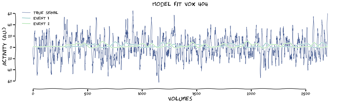
[57]:
# fit design without regressors + plot first 2 events ('left' & 'right' stimulation)
results = glm.fit_first_level(design_no_regressors, func.values, make_figure=True, xkcd=True, plot_event=[1,2])

# fit design with regressors + plot first 2 events ('left' & 'right' stimulation)
results = glm.fit_first_level(design_regressors, func.values, make_figure=True, xkcd=True, plot_event=[1, 2])
max tstat (vox 404) = 6.28
max beta (vox 404) = 3.9
max tstat (vox 478) = 7.29
max beta (vox 478) = 0.28

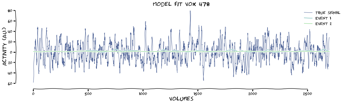
The fact that the betas drop so much after including regressors shows that my fake regressors were really bad. To help with the data structure that comes out of this function, I’ve printed the shapes of the betas and the design matrix below:
[58]:
print(f"betas have shape: {results['betas'].shape}")
print(f"design has shape: {results['x_conv'].shape}")
betas have shape: (8, 720)
design has shape: (2700, 8)
Now, we can do all of the above much easier with the GenericGLM class. First let’s repeat the fitting without regressors
[59]:
fitting = glm.GenericGLM(onsets, func.values, TR=data.TR, osf=1000, make_figure=True, xkcd=True, verbose=True, plot_event=[1,2])
Creating stimulus vector(s)
Defining HRF
Convolve stimulus vectors with HRF

Resample convolved stimulus vectors
Creating design matrix
Running fit
max tstat (vox 404) = 6.28
max beta (vox 404) = 3.9
And the design with regressors
[60]:
fitting = glm.GenericGLM(onsets, func.values, TR=data.TR, osf=1000, regressors=regressors, make_figure=True, xkcd=True, verbose=True, plot_event=[1,2])
Creating stimulus vector(s)
Defining HRF
Convolve stimulus vectors with HRF

Resample convolved stimulus vectors
Creating design matrix
Running fit
max tstat (vox 478) = 7.29
max beta (vox 478) = 0.28

[74]:
print("betas have shape: {}".format(fitting.results["betas"].shape))
print("design have shape: {}".format(fitting.results["x_conv"].shape))
betas have shape: (8, 720)
design have shape: (2700, 8)
But the shortest way is without producing plots. Just give it the onset times onsets, the fMRI-data data (either in np.ndarray form or pd.DataFrame), the TR (which can be reproduced from ParseFuncFile-object), the oversampling factor osf, and regressors (either in np.ndarray form or pd.DataFrame). Even these final 2 items (oversampling & regressors) are NOT mandatory options. They will, generally, make your analysis more accurate! Below we do the same fitting, without
regressors, but we do want the information for voxel 359 for consistency sake.
[75]:
fitting = glm.GenericGLM(onsets, func.values, TR=data.TR, osf=1000)
max tstat (vox 404) = 6.28
max beta (vox 404) = 3.9
[77]:
fitting.plot_design_matrix()