pRFmodelFitter
This page shows how I implement pRF-fitting routines on the back of prfpy. You can quite easily fit data, save data, and load data back in. It also has quick visualizations to check certain characteristics of your pRF (e.g., location in visual space, it’s raw timecourse, and the prediction given a model)
[5]:
%matplotlib inline
[2]:
from linescanning import prf, plotting, fitting
import numpy as np
import os
from scipy import io
import seaborn as sns
import matplotlib.pyplot as plt
opd = os.path.dirname
opj = os.path.join
[3]:
# first we'll load some data (I provided a npy-file in the linescanning repo)
data = np.load(opj(opd(opd(prf.__file__)), 'examples', 'prf.npy'))
data.shape
[3]:
(225, 1)
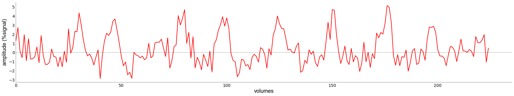
The timecourse has 225 timepoints (standard for our pRF-acquisitions) and concerns 1 voxel. We can easily plot this timecourse with LazyPlot. We can also add some customization to make the timecourse look prettier
[7]:
plotting.LazyPlot(
    data,
    add_hline="default",            # adds horizontal line at y=0
    color='r',                      # sets color of plot
    line_width=2,                   # line thickness
    x_label="volumes",              # x label
    y_label="amplitude (%signal)",  # y label
)
[7]:
<linescanning.plotting.LazyPlot at 0x7fa8de215250>
To know when the stimulus was at a given time point, we need the design matrix: a binarized representation of what happened on the screen. If you have a regular acquisition, you can use get_prfdesign to create your design matrix. For now, let’s load in the matrix we have in the repository
[8]:
# we have a .mat file, which we can load in with scipy.io.loadmat
design = io.loadmat(opj(opd(opd(prf.__file__)), 'examples', 'design_task-2R.mat'))
design
[8]:
{'__header__': b'MATLAB 5.0 MAT-file Platform: posix, Created on: Wed Jul 27 12:05:39 2022',
 '__version__': '1.0',
 '__globals__': [],
 'stim': array([[[0., 0., 0., ..., 0., 0., 0.],
         [0., 0., 0., ..., 0., 0., 0.],
         [0., 0., 0., ..., 0., 0., 0.],
         ...,
         [0., 0., 0., ..., 0., 0., 0.],
         [0., 0., 0., ..., 0., 0., 0.],
         [0., 0., 0., ..., 0., 0., 0.]],

        [[0., 0., 0., ..., 0., 0., 0.],
         [0., 0., 0., ..., 0., 0., 0.],
         [0., 0., 0., ..., 0., 0., 0.],
         ...,
         [0., 0., 0., ..., 0., 0., 0.],
         [0., 0., 0., ..., 0., 0., 0.],
         [0., 0., 0., ..., 0., 0., 0.]],

        [[0., 0., 0., ..., 0., 0., 0.],
         [0., 0., 0., ..., 0., 0., 0.],
         [0., 0., 0., ..., 0., 0., 0.],
         ...,
         [0., 0., 0., ..., 0., 0., 0.],
         [0., 0., 0., ..., 0., 0., 0.],
         [0., 0., 0., ..., 0., 0., 0.]],

        ...,

        [[0., 0., 0., ..., 0., 0., 0.],
         [0., 0., 0., ..., 0., 0., 0.],
         [0., 0., 0., ..., 0., 0., 0.],
         ...,
         [0., 0., 0., ..., 0., 0., 0.],
         [0., 0., 0., ..., 0., 0., 0.],
         [0., 0., 0., ..., 0., 0., 0.]],

        [[0., 0., 0., ..., 0., 0., 0.],
         [0., 0., 0., ..., 0., 0., 0.],
         [0., 0., 0., ..., 0., 0., 0.],
         ...,
         [0., 0., 0., ..., 0., 0., 0.],
         [0., 0., 0., ..., 0., 0., 0.],
         [0., 0., 0., ..., 0., 0., 0.]],

        [[0., 0., 0., ..., 0., 0., 0.],
         [0., 0., 0., ..., 0., 0., 0.],
         [0., 0., 0., ..., 0., 0., 0.],
         ...,
         [0., 0., 0., ..., 0., 0., 0.],
         [0., 0., 0., ..., 0., 0., 0.],
         [0., 0., 0., ..., 0., 0., 0.]]])}
[9]:
# As you can see, this is a dictionary. Not a numpy array. We can get the numpy array by selecting the `stim` attribute
design = design['stim']
print(design.shape)

# if you're not sure what the key is to find the design matrix, you can parse all the keys in the dictionary and select the last one
design = io.loadmat(opj(opd(opd(prf.__file__)), 'examples', 'design_task-2R.mat'))
key_list = list(design.keys())
print(key_list)
(100, 100, 225)
['__header__', '__version__', '__globals__', 'stim']
[10]:
# now select the last item with -1
design = design[key_list[-1]]
design.shape
[10]:
(100, 100, 225)
To make life easier, there’s a function read_par_file than can do this for you
[11]:
design = prf.read_par_file(opj(opd(opd(prf.__file__)), 'examples', 'design_task-2R.mat'))
design.shape
[11]:
(100, 100, 225)
This particular design is now a representation of the screen, but downsampled to 100x100 pixels (rather than 1920x1080) to reduce processing time. A pRF-fit generally consists of two stages: a fast search (grid-fit) in which initial parameters for the model are found and a second, slower (iterative-fit), in which we iterate over the parameters to find the optimal set. Let’s fit a simple Gaussian model.
[12]:
# the data must be <voxels,time>, but above we have <time,voxels>. We therefore need to transpose our array
gauss = prf.pRFmodelFitting(
    data.T,
    design_matrix=design,
    TR=1.5,                     # default
    model="gauss",              # default, can be 'gauss', 'css', 'dog', 'norm'
    stage="iter",               # default
    verbose=True,               # keep track of what we're doing,
    fix_bold_baseline=True      # fix the BOLD baseline at 0
)
Reading settings from '/mnt/d/FSL/shared/spinoza/programs/packages/linescanning/misc/prf_analysis.yml'
Fixing baseline at [0, 0]
Instantiate HRF with: [1, 1, 0]
The stuff above just initializes everything, rather than actually fitting it. This is so we can also load existing parameters without fitting. But, for now, let’s fit. We’ll get back to the loading later. The settings used for the grids and stuff are specified in the default settings file. Change this to your liking, but generally the defaults are fine and in compliance with Marco Aqil’s fitting procedures.
[13]:
# fit
gauss.fit()
Starting gauss grid fit at 2022/10/18 10:09:10
Completed Gaussian gridfit at 2022/10/18 10:09:19. Voxels/vertices above 0.1: 1/1
Gridfit took 0:00:08.332624
Mean rsq>0.1: 0.53
Starting gauss iterfit at 2022/10/18 10:09:19
Completed gauss iterfit at 2022/10/18 10:09:28. Mean rsq>0.1: 0.53
Iterfit took 0:00:08.940080
With plot_vox (a function inside the prf.pRFmodelFitting-object; in this case gauss), we can quickly visualize the pRF-location, the timecourse, and the predicted timecourse for a given vox_nr (especially useful if you have 2D data). It will return a tuple containing the following:
The pRF estimates
The pRF in visual field
The actual BOLD timecourse
The prediction
If you just want to see the timecourse and prf, use _,_,_,_ to silence the output. The function relies on LazyPlot and LazyPRF, so you can add the same level of customization as before, though plot_vox has some stuff set to default for you.
[14]:
# plot the model fit
_,_,_,pred1 = gauss.plot_vox(
    vox_nr=0,
    title="pars",
    axis_type="time")
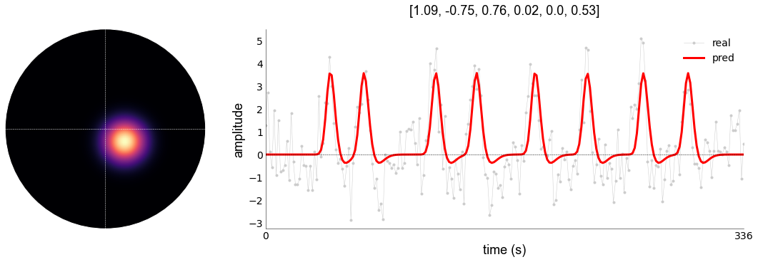
With this model, we have a variance explained of 0.53 (or 53%) percent. We can see that the baseline is indeed fixed at 0, and that the peaks generally follow the stimulation period. We can improve this by using models that capture different kinds of characteristics, such as compression (CSS), surround suppression (DoG), or both (Divisive Normalization [DN])
[15]:
# switching models is very easy. Every model that is NOT Gaussian will build on the Gaussian parameters. So, everytime your run such a model, it will re-fit the Gaussian parameters first. To avoid this, you can either specify the Gaussian fitter object (`gauss`) above as `previous_gaussian_fitter`-argument, or a numpy array as `old_params`-argument (which will create the `previous_gaussian_fitter` inside of the new object). Both options will make sure the Gaussian stage is skipped

# insert old parameters
norm = prf.pRFmodelFitting(
    data.T,
    design_matrix=design,
    TR=1.5,
    model="norm",
    stage="iter",
    verbose=True,
    fix_bold_baseline=True,
    old_params=gauss.gauss_iter, # less explicit
    )

norm = prf.pRFmodelFitting(
    data.T,
    design_matrix=design,
    TR=1.5,
    model="norm",
    stage="iter",
    verbose=True,
    fix_bold_baseline=True,
    previous_gaussian_fitter=gauss.gaussian_fitter,  # very explicit
    )

# and fit
norm.fit()
Reading settings from '/mnt/d/FSL/shared/spinoza/programs/packages/linescanning/misc/prf_analysis.yml'
Fixing baseline at [0, 0]
Instantiate HRF with: [1, 1, 0]
Reading settings from '/mnt/d/FSL/shared/spinoza/programs/packages/linescanning/misc/prf_analysis.yml'
Fixing baseline at [0, 0]
Instantiate HRF with: [1, 1, 0]
Gaussian fitter: <prfpy.fit.Iso2DGaussianFitter object at 0x7fa8de572e80>
Reading settings from '/mnt/d/FSL/shared/spinoza/programs/packages/linescanning/misc/prf_analysis.yml'
Starting norm gridfit at 2022/10/18 10:10:49
[Parallel(n_jobs=1)]: Using backend SequentialBackend with 1 concurrent workers.
[Parallel(n_jobs=1)]: Done   1 out of   1 | elapsed:    0.5s remaining:    0.0s
[Parallel(n_jobs=1)]: Done   2 out of   2 | elapsed:    0.5s remaining:    0.0s
[Parallel(n_jobs=1)]: Done   3 out of   3 | elapsed:    0.5s remaining:    0.0s
[Parallel(n_jobs=1)]: Done   4 out of   4 | elapsed:    0.5s remaining:    0.0s
[Parallel(n_jobs=1)]: Done   5 out of   5 | elapsed:    0.5s remaining:    0.0s
[Parallel(n_jobs=1)]: Done   6 out of   6 | elapsed:    0.5s remaining:    0.0s
[Parallel(n_jobs=1)]: Done   7 out of   7 | elapsed:    0.5s remaining:    0.0s
[Parallel(n_jobs=1)]: Done   8 out of   8 | elapsed:    0.5s remaining:    0.0s
[Parallel(n_jobs=1)]: Done   9 out of   9 | elapsed:    0.5s remaining:    0.0s
[Parallel(n_jobs=1)]: Done  10 out of  10 | elapsed:    0.5s remaining:    0.0s
[Parallel(n_jobs=1)]: Done 1000 out of 1000 | elapsed:    0.6s finished
Completed norm gridfit at 2022/10/18 10:10:49. Mean rsq>0.1: 0.55
Gridfit took 0:00:00.600008
Starting norm iterfit at 2022/10/18 10:10:49
Completed norm iterfit at 2022/10/18 10:14:17. Mean rsq>0.1: 0.56
Iterfit took 0:03:28.228395
[16]:
# plot the model fit
_,_,_,pred2 = norm.plot_vox(
    vox_nr=0,
    title="pars",
    model="norm")
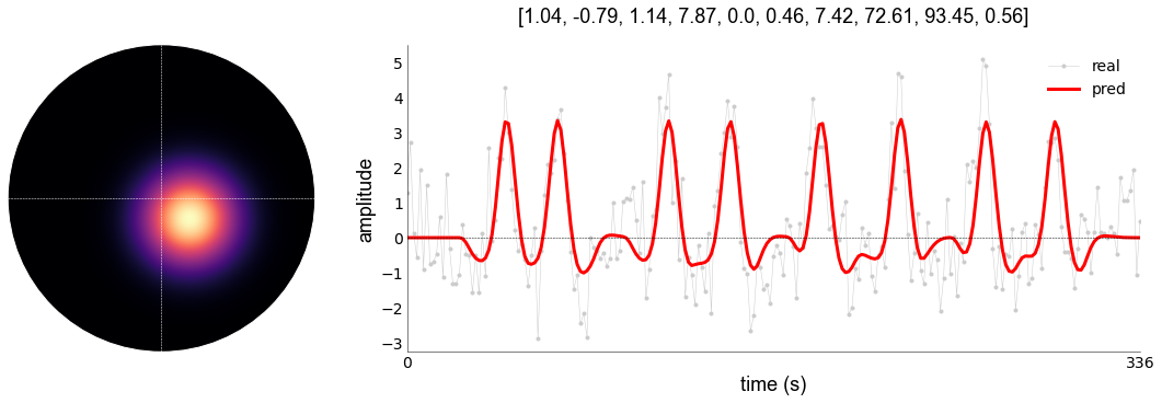
This has improved the model fit marginally. We can plot the fits together as follows:
[17]:
plotting.LazyPlot(
    [data,pred1,pred2],                       # list of multiple 1D-arrays
    add_hline="default",                      # adds horizontal line at y=0
    color=["#cccccc", 'r', "g"],              # list of same length as data (RGB/hex/strings)
    line_width=[1,2,2],                       # list of same length as data
    markers=['.',None,None],                  # plot BOLD as connected dots, predictions as solid lines
    x_label="volumes",                        # x label
    y_label="amplitude (percent signal)",     # y label
    figsize=(15,5),                           # set figure size
    labels=['BOLD','Gauss','Norm']            # labels with the same length as data list
)
[17]:
<linescanning.plotting.LazyPlot at 0x7fa8de3fc9d0>

You can see that the normalization model is capturing different characteristics compared to the Gaussian model. Also note that the processing time was a lot longer compared to the Gaussian model. These are things to consider when selecting your model (for a few hundred voxels this is fine, but for >500000 it gets a bit complicated). You can speed this up by using L-BGFS-minimization over trust-constr-minimization. See doc of `pRFmodelFitting <>`__
Now let’s look at saving and loading parameters. To save parameters, we need an output directory and the basename for the output. Some stuff will be appended depending on the stage, model, or whether the HRF was fitted as well.
[18]:
# let's use the gaussian model because it's faster
gauss = prf.pRFmodelFitting(
    data.T,
    design_matrix=design,
    TR=1.5,
    model="gauss",
    stage="iter",
    verbose=True,
    fix_bold_baseline=True,
    write_files=True,                                   # set flag to write output
    output_dir=opj(opd(opd(prf.__file__)), 'examples'), # set custom output directory (defaults to current working directory)
    output_base="sub-01_ses-1"                          # set custom output basename; "_model-{model}_stage-{stage}_desc-prf_params.{pkl|npy}" is appended
    )

# fit
gauss.fit()
Reading settings from '/mnt/d/FSL/shared/spinoza/programs/packages/linescanning/misc/prf_analysis.yml'
Fixing baseline at [0, 0]
Instantiate HRF with: [1, 1, 0]
Starting gauss grid fit at 2022/10/18 11:27:25
Completed Gaussian gridfit at 2022/10/18 11:27:34. Voxels/vertices above 0.1: 1/1
Gridfit took 0:00:09.139608
Mean rsq>0.1: 0.53
Save grid-fit parameters in /mnt/d/FSL/shared/spinoza/programs/packages/linescanning/examples/sub-01_ses-1_model-gauss_stage-grid_desc-prf_params.pkl
Starting gauss iterfit at 2022/10/18 11:27:34
Completed gauss iterfit at 2022/10/18 11:27:44. Mean rsq>0.1: 0.53
Iterfit took 0:00:09.209858
Save iter-fit parameters in /mnt/d/FSL/shared/spinoza/programs/packages/linescanning/examples/sub-01_ses-1_model-gauss_stage-iter_desc-prf_params.pkl
We see that stuff is save now in our specified directory with the basename of our choice.
[19]:
os.listdir(opj(opd(opd(prf.__file__)), 'examples'))
[19]:
['bold.mat',
 'design_task-2R.mat',
 'events.tsv',
 'figures',
 'prf.npy',
 'sub-01_ses-1_model-gauss_stage-grid_desc-prf_params.pkl',
 'sub-01_ses-1_model-gauss_stage-iter_desc-prf_params.pkl']
This pickle file has the settings, predictions, and parameters embedded in it. We can load this back in as follows:
[20]:
# we initiate the model as per usual
gauss_load = prf.pRFmodelFitting(
    data.T,
    design_matrix=design,
    TR=1.5,
    verbose=True)

# decide which parameters you want to load. Here, let's load the parameters from the iterative Gaussian fit
load_pars = opj(opj(opd(opd(prf.__file__)), 'examples'), "sub-01_ses-1_model-gauss_stage-iter_desc-prf_params.pkl")

# We would then tell `gauss_load` to load this file in, and set the correct attributes internally. If there's no known settings, it will use the most recent settings file from the directory in which the to-be-loaded parameters live. If you specify a pickle file, these default settings will be overwritten by settings specified in the pickle-file
gauss_load.load_params(load_pars, model="gauss", stage="iter")
Reading settings from '/mnt/d/FSL/shared/spinoza/programs/packages/linescanning/misc/prf_analysis.yml'
Instantiate HRF with: [1, 1, 0]
Reading settings from pickle-file (safest option; overwrites other settings)
Inserting parameters from <class 'str'> as 'gauss_iter' in <linescanning.prf.pRFmodelFitting object at 0x7fa8de225be0>
We can now make the same plot again, but from an independent object (now gauss_load, rather than gauss)
[21]:
# plot the model fit
_, _, _, pred1 = gauss_load.plot_vox(vox_nr=0, title="pars")

If we try to plot the grid-parameters, that will fail. This is because plot_vox assumes you want the iter-parameters to be plotted, but we did not set that attribute inside gauss_load
[22]:
_, _, _, _ = gauss_load.plot_vox(vox_nr=0, title='pars', stage="grid")
---------------------------------------------------------------------------
ValueError                                Traceback (most recent call last)
/tmp/ipykernel_710/2874508505.py in <module>
----> 1 _, _, _, _ = gauss_load.plot_vox(vox_nr=0, title='pars', stage="grid")

/mnt/d/FSL/shared/spinoza/programs/packages/linescanning/linescanning/prf.py in plot_vox(self, vox_nr, model, stage, make_figure, xkcd, title, transpose, freq_spectrum, freq_type, clip_power, save_as, axis_type, resize_pix, add_tc, axs, **kwargs)
   2146                 raise ValueError(f"Array of length {len(vox_nr)} was given. Can only be 1")
   2147
-> 2148         self.prediction, params, vox = self.make_predictions(
   2149             vox_nr=vox_nr,
   2150             model=model,

/mnt/d/FSL/shared/spinoza/programs/packages/linescanning/linescanning/prf.py in make_predictions(self, vox_nr, model, stage)
   2037
   2038         else:
-> 2039             raise ValueError(f"Could not find {stage} parameters for {model}")
   2040
   2041     def plot_vox(

ValueError: Could not find grid parameters for gauss
It will also fail if we try to plot a model other than the one we specified (in our case, gauss), because we told the object to load in the parameters as gauss.
[23]:
_, _, _, _ = gauss_load.plot_vox(vox_nr=0, title='pars', stage="iter", model="norm")
---------------------------------------------------------------------------
ValueError                                Traceback (most recent call last)
/tmp/ipykernel_710/2886960258.py in <module>
----> 1 _, _, _, _ = gauss_load.plot_vox(vox_nr=0, title='pars', stage="iter", model="norm")

/mnt/d/FSL/shared/spinoza/programs/packages/linescanning/linescanning/prf.py in plot_vox(self, vox_nr, model, stage, make_figure, xkcd, title, transpose, freq_spectrum, freq_type, clip_power, save_as, axis_type, resize_pix, add_tc, axs, **kwargs)
   2146                 raise ValueError(f"Array of length {len(vox_nr)} was given. Can only be 1")
   2147
-> 2148         self.prediction, params, vox = self.make_predictions(
   2149             vox_nr=vox_nr,
   2150             model=model,

/mnt/d/FSL/shared/spinoza/programs/packages/linescanning/linescanning/prf.py in make_predictions(self, vox_nr, model, stage)
   2037
   2038         else:
-> 2039             raise ValueError(f"Could not find {stage} parameters for {model}")
   2040
   2041     def plot_vox(

ValueError: Could not find iter parameters for norm
Finally, we can also fit the HRF-parameters during the pRF-modeling. This is handy if you expect differing HRFs across regions (or cortical depth). If you’re doing this with models other than the Gaussian model, it’s advised to do this in two stages:
Fit your data without fitting the HRF
Then insert these parameters into a fit with HRF fitting
This is to avoid sending the fitter into the forest without a maps, as adding more parameters to a model increases model complexity. Given existing parameters to the fitter will tame the optimizer.
[24]:
# stage 1: no HRF
stage1 = prf.pRFmodelFitting(
    data.T,
    design_matrix=design,
    TR=1.5,
    model="norm",
    stage="grid+iter",
    verbose=True,
    fix_bold_baseline=True
    )

stage1.fit()

# stage 2: HRF with estimates from stage1
stage2 = prf.pRFmodelFitting(
    data.T,
    design_matrix=design,
    TR=1.5,
    model="norm",
    stage="iter",
    verbose=True,
    fix_bold_baseline=True,
    fit_hrf=True,                                  # fit HRF,
    previous_gaussian_fitter=stage1.norm_fitter    # give existing parameters
    )

stage2.fit()
Reading settings from '/mnt/d/FSL/shared/spinoza/programs/packages/linescanning/misc/prf_analysis.yml'
Fixing baseline at [0, 0]
Instantiate HRF with: [1, 1, 0]
Starting gauss grid fit at 2022/10/18 11:29:42
Completed Gaussian gridfit at 2022/10/18 11:29:51. Voxels/vertices above 0.1: 1/1
Gridfit took 0:00:09.080517
Mean rsq>0.1: 0.53
Starting gauss iterfit at 2022/10/18 11:29:51
Completed gauss iterfit at 2022/10/18 11:30:00. Mean rsq>0.1: 0.53
Iterfit took 0:00:09.047231
Reading settings from '/mnt/d/FSL/shared/spinoza/programs/packages/linescanning/misc/prf_analysis.yml'
Starting norm gridfit at 2022/10/18 11:30:00
[Parallel(n_jobs=1)]: Using backend SequentialBackend with 1 concurrent workers.
[Parallel(n_jobs=1)]: Done   1 out of   1 | elapsed:    0.4s remaining:    0.0s
[Parallel(n_jobs=1)]: Done   2 out of   2 | elapsed:    0.4s remaining:    0.0s
[Parallel(n_jobs=1)]: Done   3 out of   3 | elapsed:    0.4s remaining:    0.0s
[Parallel(n_jobs=1)]: Done   4 out of   4 | elapsed:    0.4s remaining:    0.0s
[Parallel(n_jobs=1)]: Done   5 out of   5 | elapsed:    0.4s remaining:    0.0s
[Parallel(n_jobs=1)]: Done   6 out of   6 | elapsed:    0.4s remaining:    0.0s
[Parallel(n_jobs=1)]: Done   7 out of   7 | elapsed:    0.4s remaining:    0.0s
[Parallel(n_jobs=1)]: Done   8 out of   8 | elapsed:    0.4s remaining:    0.0s
[Parallel(n_jobs=1)]: Done   9 out of   9 | elapsed:    0.4s remaining:    0.0s
[Parallel(n_jobs=1)]: Done  10 out of  10 | elapsed:    0.4s remaining:    0.0s
[Parallel(n_jobs=1)]: Done 1000 out of 1000 | elapsed:    0.5s finished
Completed norm gridfit at 2022/10/18 11:30:00. Mean rsq>0.1: 0.55
Gridfit took 0:00:00.555609
Starting norm iterfit at 2022/10/18 11:30:00
Completed norm iterfit at 2022/10/18 11:33:45. Mean rsq>0.1: 0.56
Iterfit took 0:03:44.880959
Reading settings from '/mnt/d/FSL/shared/spinoza/programs/packages/linescanning/misc/prf_analysis.yml'
Fixing baseline at [0, 0]
Instantiate HRF with: [1, 1, 0]
Gaussian fitter: <prfpy.fit.Norm_Iso2DGaussianFitter object at 0x7fa8de288f40>
Reading settings from '/mnt/d/FSL/shared/spinoza/programs/packages/linescanning/misc/prf_analysis.yml'
Starting norm gridfit at 2022/10/18 11:33:46
[Parallel(n_jobs=1)]: Using backend SequentialBackend with 1 concurrent workers.
[Parallel(n_jobs=1)]: Done   1 out of   1 | elapsed:    0.4s remaining:    0.0s
[Parallel(n_jobs=1)]: Done   2 out of   2 | elapsed:    0.4s remaining:    0.0s
[Parallel(n_jobs=1)]: Done   3 out of   3 | elapsed:    0.4s remaining:    0.0s
[Parallel(n_jobs=1)]: Done   4 out of   4 | elapsed:    0.4s remaining:    0.0s
[Parallel(n_jobs=1)]: Done   5 out of   5 | elapsed:    0.4s remaining:    0.0s
[Parallel(n_jobs=1)]: Done   6 out of   6 | elapsed:    0.4s remaining:    0.0s
[Parallel(n_jobs=1)]: Done   7 out of   7 | elapsed:    0.4s remaining:    0.0s
[Parallel(n_jobs=1)]: Done   8 out of   8 | elapsed:    0.4s remaining:    0.0s
[Parallel(n_jobs=1)]: Done   9 out of   9 | elapsed:    0.4s remaining:    0.0s
[Parallel(n_jobs=1)]: Done  10 out of  10 | elapsed:    0.4s remaining:    0.0s
[Parallel(n_jobs=1)]: Done 1000 out of 1000 | elapsed:    0.5s finished
Completed norm gridfit at 2022/10/18 11:33:46. Mean rsq>0.1: 0.56
Gridfit took 0:00:00.493177
Starting norm iterfit at 2022/10/18 11:33:46
Completed norm iterfit at 2022/10/18 11:41:56. Mean rsq>0.1: 0.63
Iterfit took 0:08:10.164019
[25]:
# plot the model fit
_, _, _, no_hrf = stage1.plot_vox(
    vox_nr=0,
    title="pars",
    model="norm")

_, _, _, with_hrf = stage2.plot_vox(
    vox_nr=0,
    title="pars",
    model="norm"
)

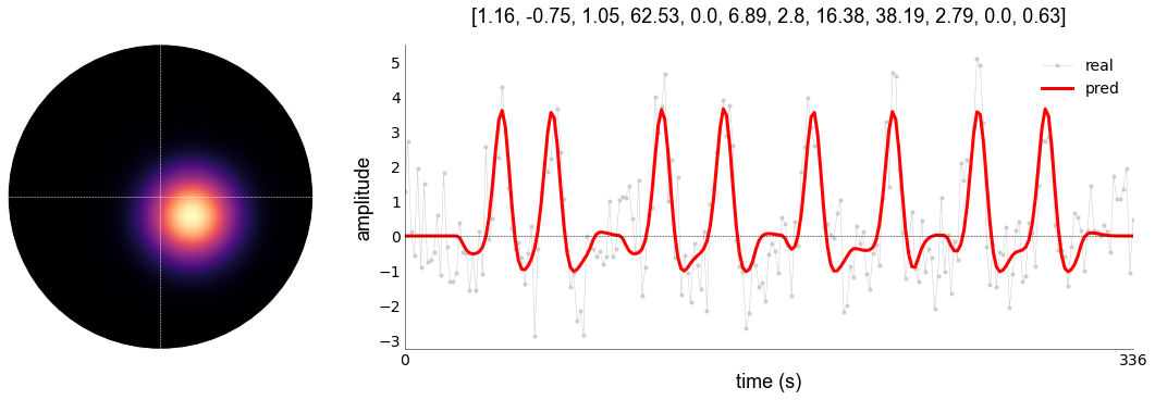
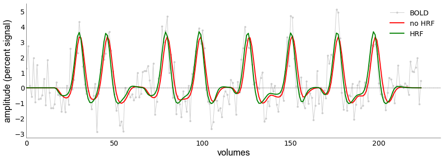
Again, you see that adding the HRF results in improved variance explained (r2): 0.56 vs 0.63.
[27]:
plotting.LazyPlot(
    [data,no_hrf,with_hrf],
    add_hline="default",
    color=["#cccccc", 'r', "g"],
    line_width=[1,2,2],
    markers=['.',None,None],
    x_label="volumes",
    y_label="amplitude (percent signal)",
    labels=['BOLD','no HRF','HRF'],
    figsize=(15,5))
[27]:
<linescanning.plotting.LazyPlot at 0x7fa8dc18bf10>
We can also plot the HRFs
[29]:
fig,axs = plt.subplots(figsize=(8,8))

# HRF is now created inside the object (a new feature of pRFpy)
stage1.hrf.create_spm_hrf(hrf_params=[1,1,0], TR=stage1.TR, force=True)
stage2.hrf.create_spm_hrf(hrf_params=[1, *stage2.norm_iter[0, -3:-1]], TR=stage1.TR, force=True)

hrfs = [stage1.hrf.values.T, stage2.hrf.values.T]
plotting.LazyPlot(
    hrfs,
    labels=["standard HRF","Fitted HRF"],
    xx=np.arange(0,40,stage2.TR),             # custom x-axis
    axs=axs,                                  # give existing axis to `LazyPlot` > allows you to put LazyPlot figures on different subplot axes
    label_size=14,
    font_size=18,
    line_width=2,
    x_lim=[0,25],
    add_hline='default',
    cmap='inferno',                           # custom color map
    x_label="time (s)",
    y_label="magnitude")

# get fwhm
colors = sns.color_palette('inferno', len(hrfs))
fwhm_objs = []
for hrf in hrfs:
    fwhm_objs.append(fitting.FWHM(np.arange(0,40,stage2.TR), hrf))

    # heights need to be adjusted for by axis length
    xlim = axs.get_xlim()
    tot = sum(list(np.abs(xlim)))
    for ix, ii in enumerate(fwhm_objs):
        start = (ii.hmx[0]-xlim[0])/tot
        axs.axhline(ii.half_max, xmin=start, xmax=start+ii.fwhm/tot, color=colors[ix], linewidth=0.5)
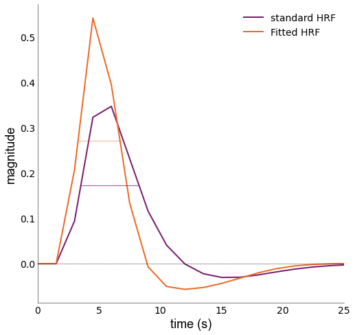
We can see that the Fitted HRF is faster than the standard HRF; something would expect from 7T data